Highway Lane Following
This example shows how to simulate a highway lane following application with vision processing, sensor fusion, and controller components. These components are tested in a 3D simulation environment that includes camera and radar sensor models.
Introduction
A highway lane following system steers a vehicle to travel within a marked lane. It also maintains a set velocity or safe distance to a preceding vehicle in the same lane. The system typically uses vision processing algorithms to detect lanes and vehicles from a camera. The vehicle detections from the camera are then fused with detections from a radar to improve the robustness of perception. The controller uses the lane detections, vehicle detections, and set speed to control steering and acceleration.
This example demonstrates how to create a test bench model to test vision processing, sensor fusion, and controls in a 3D simulation environment. The test bench model can be configured for different scenarios to test the ability to follow lanes and avoid collisions with other vehicles. In this example, you:
Partition the algorithm and test bench — The model is partitioned into lane following algorithm models and a test bench model. The algorithm models implement the individual components. The test bench includes the integration of the algorithm models, and virtual testing framework.
Explore the test bench model — The test bench model contains the testing framework, which includes the scenario, ego vehicle dynamics model, and metrics assessment using ground truth. A cuboid scenario defines vehicle trajectories and specifies the ground truth. An equivalent Unreal Engine® scene is used to model detections from a radar sensor and images from a monocular camera sensor. A bicycle model is used to model the ego vehicle.
Explore the algorithm models — Algorithm models are reference models that implement vision processing, sensor fusion, decision logic, and controls components to build the lane following application.
Visualize a test scenario — The scenario contains a curved road with multiple vehicles.
Simulate the test bench model — The model is simulated to test integration of the vision processing, sensor fusion, and controls components.
Explore additional scenarios — These scenarios test the system under additional conditions.
Testing the integration of the controller and the perception algorithm requires a photorealistic simulation environment. In this example, you enable system-level simulation through integration with the Unreal Engine from Epic Games®.
if ~ispc
    error(['This example is supported only on Microsoft', char(174), ...
        ' Windows', char(174), '.'])
end
To ensure reproducibility of the simulation results, set the random seed.
rng(0)
Partition Algorithm and Test Bench
The model is partitioned into separate algorithm and test bench models.
Algorithm models — Algorithm models are reference models that implement the functionality of individual components.
Test bench model — The Highway Lane Following test bench specifies the stimulus and environment to test the algorithm models.
Explore Test Bench Model
In this example, you use a system-level simulation test bench model to explore the behavior of the control and vision processing algorithms for the lane following system.
To explore the test bench model, load the highway lane following project.
openProject("HighwayLaneFollowing");
Open the system-level simulation test bench model.
open_system("HighwayLaneFollowingTestBench")

The test bench model contains these modules:
Simulation 3D Scenario — Subsystem that specifies the road, vehicles, camera sensor, and radar sensor used for simulation.
Lane Marker Detector — Algorithm model to detect the lane boundaries in the frame captured by the camera sensor.
Vehicle Detector — Algorithm model to detect vehicles in the frame captured by the camera sensor.
Forward Vehicle Sensor Fusion — Algorithm model to fuse vehicle detections from the camera and radar sensors.
Lane Following Decision Logic — Algorithm model to specify the lateral and longitudinal decision logic that provides information related to the most important object (MIO) and lane center to the controller.
Lane Following Controller — Algorithm model that specifies the steering angle and acceleration controls.
Vehicle Dynamics — Subsystem that specifies the dynamic model of the ego vehicle.
Metrics Assessment — Subsystem that assesses system-level and component-level behaviors.
The Simulation 3D Scenario subsystem configures the road network, positions vehicles, and synthesizes sensors. Open the Simulation 3D Scenario subsystem.
open_system("HighwayLaneFollowingTestBench/Simulation 3D Scenario")
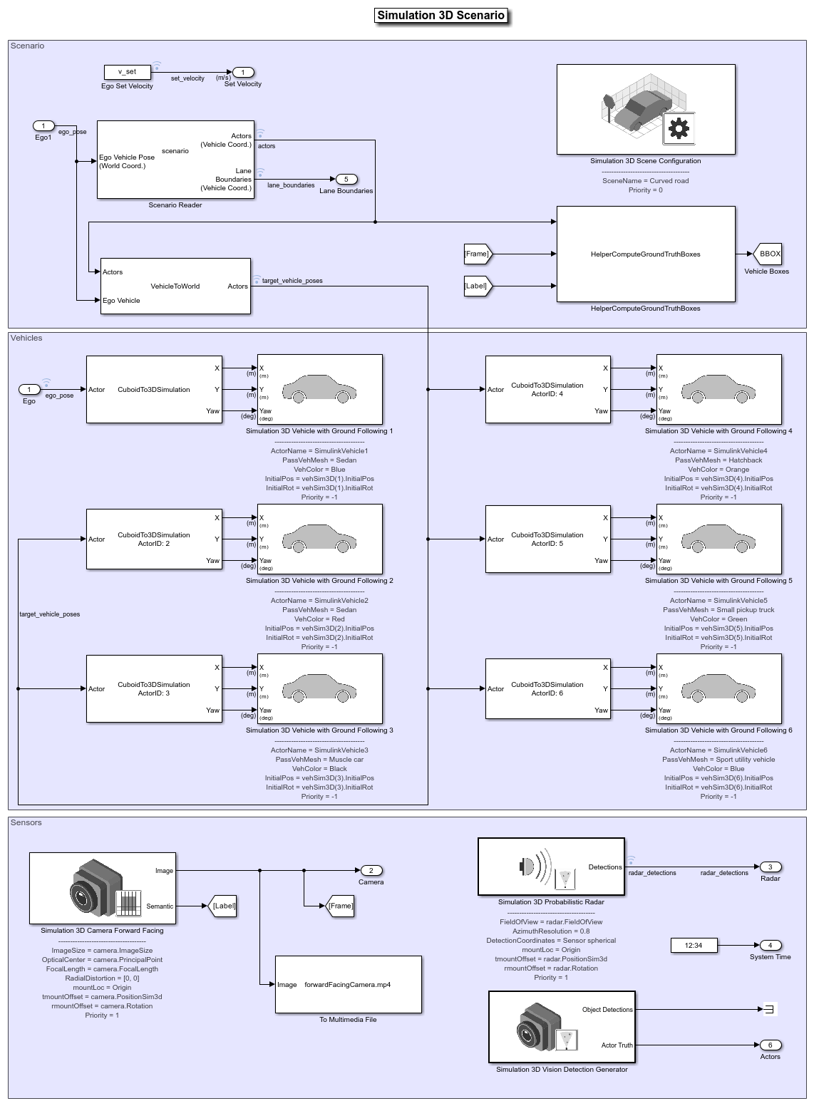
The scene and road network are specified by these parts of the subsystem:
The Simulation 3D Scene Configuration (Automated Driving Toolbox) block has the SceneName parameter set to
Curved road.The Scenario Reader (Automated Driving Toolbox) block is configured to use a driving scenario that contains a road network that closely matches a section of the road network from the
Curved roadscene.
The vehicle positions are specified by these parts of the subsystem:
The Ego input port controls the position of the ego vehicle, which is specified by the Simulation 3D Vehicle with Ground Following 1 block.
The Vehicle To World (Automated Driving Toolbox) block converts actor poses from the coordinates of the ego vehicle to the world coordinates.
The Scenario Reader (Automated Driving Toolbox) block outputs actor poses, which control the position of the target vehicles. These vehicles are specified by the other Simulation 3D Vehicle with Ground Following (Automated Driving Toolbox) blocks.
The Cuboid To 3D Simulation (Automated Driving Toolbox) block converts the ego pose coordinate system (with respect to below the center of the vehicle rear axle) to the 3D simulation coordinate system (with respect to below the vehicle center).
The
HeplerComputeGroundTruthBoxesSystem object™ computes the ground truth vehicle bounding boxes using actual actor positions received from the Scenario Reader (Automated Driving Toolbox) block and labeled image data received from the Simulation 3D Camera (Automated Driving Toolbox) block.
The sensors attached to the ego vehicle are specified by these parts of the subsystem:
The Simulation 3D Camera (Automated Driving Toolbox) block is attached to the ego vehicle to capture its front view. The output image from this block is processed by the Lane Marker Detector block to detect the lanes and Vehicle Detector block to detect the vehicles.
The Simulation 3D Probabilistic Radar (Automated Driving Toolbox) block is attached to the ego vehicle to detect vehicles in 3D simulation environment.
The Simulation 3D Vision Detection Generator (Automated Driving Toolbox) block generates the actor position truth from the from camera measurements taken by a vision sensor mounted on an ego vehicle in a 3D simulation environment.
The Vehicle Dynamics subsystem uses a Bicycle Model block to model the ego vehicle. Open the Vehicle Dynamics subsystem.
open_system("HighwayLaneFollowingTestBench/Vehicle Dynamics");
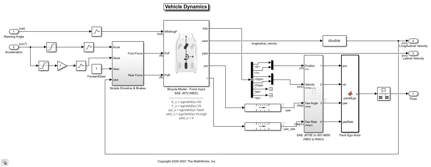
The Bicycle Model block implements a rigid two-axle single track vehicle body model to calculate longitudinal, lateral, and yaw motion. The block accounts for body mass, aerodynamic drag, and weight distribution between the axles due to acceleration and steering. For more details, see Bicycle Model (Automated Driving Toolbox).
The Metrics Assessment subsystem enables system-level and component-level metric evaluations using the ground truth information from the scenario. Open the Metrics Assessment subsystem.
open_system("HighwayLaneFollowingTestBench/Metrics Assessment");

Using this example, you can evaluate the system-level behavior using four system-level metrics. Additionally, you can also compute component-level metrics to analyze individual components and their impact on the overall system performance.
System-Level Metrics
Verify Lateral Deviation — This block verifies that the lateral deviation from the center line of the lane is within prescribed thresholds for the corresponding scenario. Define the thresholds when you author the test scenario.
Verify In Lane — This block verifies that the ego vehicle is following one of the lanes on the road throughout the simulation.
Verify Time gap — This block verifies that the time gap between the ego vehicle and the lead vehicle is more than 0.8 seconds. The time gap between the two vehicles is defined as the ratio of the calculated headway distance to the ego vehicle velocity.
Verify No Collision — This block verifies that the ego vehicle does not collide with the lead vehicle at any point during the simulation.
Component-Level Metrics
Lane Metrics — This block verifies that distances between the detected lane boundaries and the ground truth data are within the thresholds specified in a test scenario.
Vehicle Detector Metrics — This blocks computes and logs true positives, false negatives, and false positives for the detections.
Sensor Fusion & Tracking Metrics — This subsystem computes generalized optimal subpattern assignment (GOSPA) metric, localization error, missed target error, and false track error. For more information on these metrics, see Forward Vehicle Sensor Fusion (Automated Driving Toolbox) example.
You can integrate these metrics with Simulink Test™ and enable automatic regression testing. For more information, see Automate Testing for Highway Lane Following (Automated Driving Toolbox) example.
Explore Algorithm Models
The lane following system is developed by integrating the lane marker detector, vehicle detector, forward vehicle sensor fusion, lane following decision logic, and lane following controller components.
The lane marker detector algorithm model implements a perception module to analyze the images of roads. Open the Lane Marker Detector algorithm model.
open_system("LaneMarkerDetector");
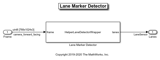
The lane marker detector takes the frame captured by a monocular camera sensor as input. It also takes in the camera intrinsic parameters through the mask. It detects the lane boundaries and outputs the lane information and marking type of each lane through the LaneSensor bus. For more details on how to design and evaluate a lane marker detector, see Design Lane Marker Detector Using Unreal Engine Simulation Environment (Automated Driving Toolbox) and Generate Code for Lane Marker Detector (Automated Driving Toolbox).
The vehicle detector algorithm model detects vehicles in the driving scenario. Open the Vehicle Detector algorithm model.
open_system("VisionVehicleDetector");
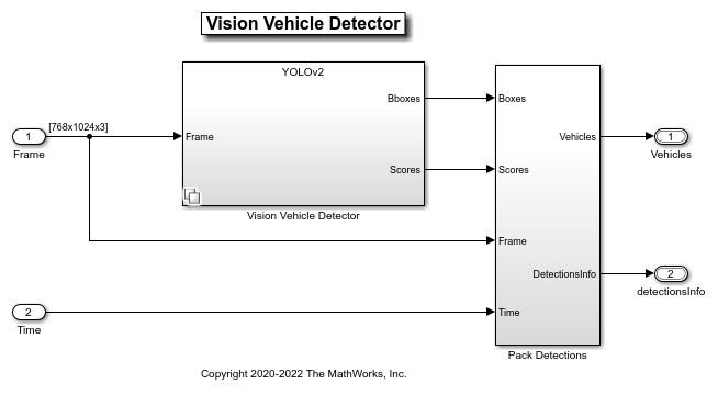
The vehicle detector takes the frame captured by a camera sensor as input. It also takes in the camera intrinsic parameters through the mask. It detects the vehicles and outputs the vehicle information as bounding boxes. For more details on how to design and evaluate a vehicle detector, see Generate Code for Vision Vehicle Detector (Automated Driving Toolbox).
The forward vehicle sensor fusion component fuses the vehicle detections from camera and radar sensors and tracks the detected vehicles using the central level tracking method. Open the Forward Vehicle Sensor Fusion algorithm model.
open_system("ForwardVehicleSensorFusion");
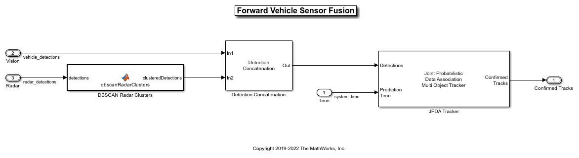
The forward vehicle sensor fusion model takes in the vehicle detections from vision and radar sensors as inputs. The radar detections are clustered and then concatenated with vision detections. The concatenated vehicle detections are then tracked using a joint probabilistic data association tracker. This component outputs the confirmed tracks. For more details on forward vehicle sensor fusion, see Forward Vehicle Sensor Fusion (Automated Driving Toolbox).
The lane following decision logic algorithm model specifies lateral and longitudinal decisions based on the detected lanes and tracks. Open the Lane Following Decision Logic algorithm model.
open_system("LaneFollowingDecisionLogic");
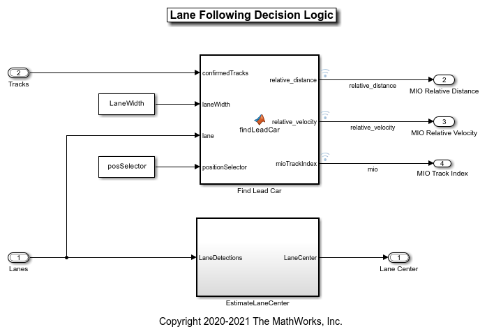
The lane following decision logic model takes the detected lanes from the lane marker detector and the confirmed tracks from the forward vehicle sensor fusion module as inputs. It estimates the lane center and also determines the MIO lead car traveling in the same lane as the ego vehicle. It outputs the relative distance and relative velocity between the MIO and ego vehicle.
The lane following controller specifies the longitudinal and lateral controls. Open the Lane Following Controller algorithm model.
open_system("LaneFollowingController");

The controller takes the set velocity, lane center, and MIO information as inputs. It uses a path following controller to control the steering angle and acceleration for the ego vehicle. It also uses a watchdog braking controller to apply brakes as a fail-safe mode. The controller outputs the steering angle and acceleration command that determines whether to accelerate, decelerate, or apply brakes. The Vehicle Dynamics block uses these outputs for lateral and longitudinal control of the ego vehicle.
Visualize Test Scenario
The helper function scenario_LFACC_03_Curve_StopnGo generates a cuboid scenario that is compatible with the HighwayLaneFollowingTestBench model. This is an open-loop scenario containing multiple target vehicles on a curved road. The road centers, lane markings, and vehicles in this cuboid scenario closely match a section of the curved road scene provided with the 3D simulation environment. In this scenario, a lead vehicle slows down in front of the ego vehicle while other vehicles travel in adjacent lanes.
Plot the open-loop scenario to see the interactions of the ego vehicle and target vehicles.
hFigScenario = helperPlotLFScenario("scenario_LFACC_03_Curve_StopnGo");
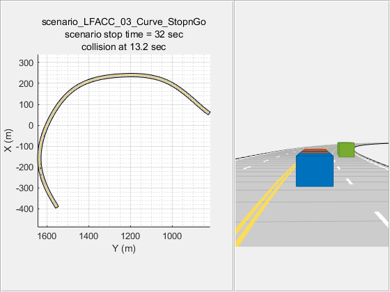
The ego vehicle is not under closed-loop control, so a collision occurs with the slower moving lead vehicle. The goal of the closed-loop system is to follow the lane and maintain a safe distance from the lead vehicles. In the HighwayLaneFollowingTestBench model, the ego vehicle has the same initial velocity and initial position as in the open-loop scenario.
Close the figure.
close(hFigScenario)
Simulate Test Bench Model
Configure and test the integration of the algorithms in the 3D simulation environment. To reduce command-window output, turn off the MPC update messages.
mpcverbosity("off");
Configure the test bench model to use the same scenario.
helperSLHighwayLaneFollowingSetup("scenarioFcnName",...
    "scenario_LFACC_03_Curve_StopnGo");
sim("HighwayLaneFollowingTestBench")
Plot the lateral controller performance results.
hFigLatResults = helperPlotLFLateralResults(logsout);

Close the figure.
close(hFigLatResults)
Examine the simulation results.
The Detected lane boundary lateral offsets plot shows the lateral offsets of the detected left-lane and right-lane boundaries from the centerline of the lane. The detected values are close to the ground truth of the lane but deviate by small quantities.
The Lateral deviation plot shows the lateral deviation of the ego vehicle from the centerline of the lane. Ideally, lateral deviation is zero meters, which implies that the ego vehicle exactly follows the centerline. Small deviations occur when the vehicle is changing velocity to avoid collision with another vehicle.
The Relative yaw angle plot shows the relative yaw angle between ego vehicle and the centerline of the lane. The relative yaw angle is very close to zero radian, which implies that the heading angle of the ego vehicle matches the yaw angle of the centerline closely.
The Steering angle plot shows the steering angle of the ego vehicle. The steering angle trajectory is smooth.
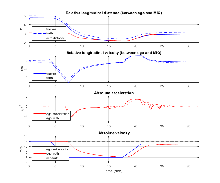
Plot the longitudinal controller performance results.
hFigLongResults = helperPlotLFLongitudinalResults(logsout,time_gap,...
    default_spacing);
Close the figure.
close(hFigLongResults)
Examine the simulation results.
The Relative longitudinal distance plot shows the distance between the ego vehicle and the MIO. In this case, the ego vehicle approaches the MIO and gets close to it or exceeds the safe distance in some cases.
The Relative longitudinal velocity plot shows the relative velocity between the ego vehicle and the MIO. In this example, the vehicle detector only detects positions, so the tracker in the control algorithm estimates the velocity. The estimated velocity lags the actual (ground truth) MIO relative velocity.
The Absolute acceleration plot shows that the controller commands the vehicle to decelerate when it gets too close to the MIO.
The Absolute velocity plot shows the ego vehicle initially follows the set velocity, but when the MIO slows down, to avoid a collision, the ego vehicle also slows down.
During simulation, the model logs signals to the base workspace as logsout and records the output of the camera sensor to forwardFacingCamera.mp4. You can use the helperPlotLFDetectionResults function to visualize the simulated detections similar to how recorded data is explored in the Forward Collision Warning Using Sensor Fusion (Automated Driving Toolbox) example. You can also record the visualized detections to a video file to enable review by others who do not have access to MATLAB.
Plot the detection results from logged data, generate a video, and open the Video Viewer (Image Processing Toolbox) app.
hVideoViewer = helperPlotLFDetectionResults(...
    logsout, "forwardFacingCamera.mp4" , scenario, camera, radar,...
    scenarioFcnName,...
    "RecordVideo", true,...
    "RecordVideoFileName", scenarioFcnName + "_VPA",...
    "OpenRecordedVideoInVideoViewer", true,...
    "VideoViewerJumpToTime", 10.6);

Play the generated video.
Front Facing Camera shows the image returned by the camera sensor. The left lane boundary is plotted in red and the right lane boundary is plotted in green. These lanes are returned by the Lane Marker Detector model. Tracked detections are also overlaid on the video.
Bird's-Eye Plot shows true vehicle positions, sensor coverage areas, probabilistic detections, and track outputs. The plot title includes the simulation time so that you can correlate events between the video and previous static plots.
Close the figure.
close(hVideoViewer)
Explore Additional Scenarios
The previous simulations tested the scenario_LFACC_03_Curve_StopnGo scenario. This example provides additional scenarios that are compatible with the HighwayLaneFollowingTestBench model:
  scenario_LF_01_Straight_RightLane
  scenario_LF_02_Straight_LeftLane
  scenario_LF_03_Curve_LeftLane
  scenario_LF_04_Curve_RightLane
  scenario_LFACC_01_Curve_DecelTarget
  scenario_LFACC_02_Curve_AutoRetarget
  scenario_LFACC_03_Curve_StopnGo
  scenario_LFACC_04_Curve_CutInOut
  scenario_LFACC_05_Curve_CutInOut_TooClose
  scenario_LFACC_06_Straight_StopandGoLeadCar
These scenarios represent two types of testing.
Use scenarios with the
scenario_LF_prefix to test lane-detection and lane-following algorithms without obstruction from other vehicles. The vehicles in the scenario are positioned such that they are not seen by the ego vehicle.Use scenarios with the
scenario_LFACC_prefix to test lane-detection and lane-following algorithms with other vehicles that are within the sensor coverage area of the ego vehicle.
Examine the comments in each file for more details about the geometry of the road and vehicles in each scenario. You can configure the HighwayLaneFollowingTestBench model and workspace to simulate these scenarios using the helperSLHighwayLaneFollowingSetup function.
For example, while evaluating the effects of a camera-based lane detection algorithm on closed-loop control, it can be helpful to begin with a scenario that has a road but no vehicles. To configure the model and workspace for such a scenario, use the following code.
helperSLHighwayLaneFollowingSetup("scenarioFcnName",...
    "scenario_LF_04_Curve_RightLane");
Enable the MPC update messages again.
mpcverbosity("on");
Conclusion
This example showed how to integrate vision processing, sensor fusion and controller components to simulate a highway lane following system in a closed-loop 3D simulation environment. The example also demonstrated various evaluation metrics to validate the performance of the designed system. If you have licenses for Simulink Coder™ and Embedded Coder™ you can generate ready to deploy code with the embedded real-time target (ERT).
See Also
Blocks
Related Examples
More About
You can also select a web site from the following list:
Americas
- América Latina (Español)
- Canada (English)
- United States (English)
Europe
- Belgium (English)
- Denmark (English)
- Deutschland (Deutsch)
- España (Español)
- Finland (English)
- France (Français)
- Ireland (English)
- Italia (Italiano)
- Luxembourg (English)
- Netherlands (English)
- Norway (English)
- Österreich (Deutsch)
- Portugal (English)
- Sweden (English)
- Switzerland
- United Kingdom (English)