Parallel Parking Using Nonlinear Model Predictive Control
This example shows how to design a parallel parking controller using nonlinear model predictive control (NLMPC).
Parking Environment
In this example, the parking environment contains an ego vehicle and six static obstacles. The obstacles include four parked vehicles, the road curbside, and a yellow line on the road. The goal of the ego vehicle is to park at a target pose without colliding with any of the obstacles. The reference point for the ego vehicle pose is located at the center of rear axle.
The ego vehicle has two axles and four wheels. Define the ego vehicle parameters.
vdims = vehicleDimensions;
egoWheelbase = vdims.Wheelbase;
distToCenter = 0.5*egoWheelbase;
The ego vehicle starts at the following initial pose.
X position of
7mY position of
3.1mYaw angle
0rad
egoInitialPose = [7,3.1,0];
To park the center of the ego vehicle at the target location (X = 0, Y = 0) use the following target pose, which specifies the location of the rear-axle reference point.
X position equal to half the wheelbase length in the negative X direction
Y position of
0mYaw angle
0rad
egoTargetPose = [-distToCenter,0,0];
Visualize the parking environment. Specify a visualizer sample time of 0.1 s.
Tv = 0.1;
helperSLVisualizeParking(egoInitialPose,0);

In the visualization, the four parked vehicles are the orange boxes in the middle. The bottom orange boundary is the road curbside and the top orange boundary is the yellow line on the road.
Ego Vehicle Model
For parking problems, the vehicle travels at low speeds. This example uses a kinematic bicycle model with front steering angle for the vehicle parking problem. The motion of the ego vehicle can be described using the following equations.
Here, denotes the position of the vehicle and denotes the yaw angle of the vehicle. The parameter represents the wheelbase of the vehicle. are the state variables for the vehicle state functions. The speed and steering angle are the control variables for the vehicle state functions. The vehicle state functions are implemented in parkingVehicleStateFcn.
Design a Path Planner Using Nonlinear Model Predictive Controller
The nonlinear model predictive controller for parking is designed based on the following analysis.
The output of the vehicle state function is the same as the state of the vehicle . Therefore, the NLMPC controller is created with three states, three outputs, and two manipulated variables.
The speed of the ego vehicle is constrained to be between -2 and 2 m/s, and the steering angle of the ego vehicle is constrained to be between -45 and 45 degrees.
The NLMPC controller uses a custom cost function, which is defined in a manner similar to a quadratic tracking cost plus a terminal cost. In the following custom cost function, denotes the states of ego vehicle at time , represents the duration of simulation, and is the target pose of the ego vehicle. The weight matrices , , , and are constant.
To avoid collisions with obstacles, the NLMPC controller must satisfy the following inequality constraints where the minimum distance to all obstacles must be greater than a safe distance . In this example, the ego vehicle and obstacles are modeled as
collisionBox(Robotics System Toolbox) objects and the distance from ego vehicle to obstacles is computed usingcheckCollision(Robotics System Toolbox).
To improve the computation efficiency, the Jacobians of the state function, cost function, and inequality constraints are all provided to the NLMPC controller. The Jacobians of the inequality constraints are approximated based on [1].
The initial guesses for the state solutions are defined by straight lines between the initial and target poses of the ego vehicle.
Specify the sample time (Ts), prediction horizon (p), and control horizon (m) for the nonlinear MPC controller. The prediction time, which is the prediction horizon multiplied by sample time, is 5 seconds implying that the planner can make the vehicle reach the desired pose by 5 seconds.
Ts = 0.1;
p = 50;
c = 50;
Specify constant weight matrices for the controller. Define both the tracking weight matrices (Qp and Rp) and the terminal weight matrices (Qt and Rt).
Qp = diag([0.1 0.1 0]);
Rp = 0.01*eye(2);
Qt = diag([1 5 100]);
Rt = 0.1*eye(2);
Specify the safety distance of 0.1 m, which the controller uses when defining its constraints.
safetyDistance = 0.1;
Create the nonlinear MPC controller. For clarity, first disable the MPC command-window messages.
mpcverbosity('off');Create the nlmpc controller object with three states, three outputs, and two inputs.
nx = 3;
ny = 3;
nu = 2;
nlobj = nlmpc(nx,ny,nu);
Specify the sample time (Ts), prediction horizon (PredictionHorizon), and control horizon (ControlHorizon) for the controller.
nlobj.Ts = Ts;
nlobj.PredictionHorizon = p;
nlobj.ControlHorizon = c;
Define constraints for the manipulated variables. Here, MV(1) is the ego vehicle speed in m/s, and MV(2) is the steering angle in radians.
nlobj.MV(1).Min = -2;
nlobj.MV(1).Max = 2;
nlobj.MV(2).Min = -pi/4;
nlobj.MV(2).Max = pi/4;
Specify the controller state function and the state-function Jacobian.
nlobj.Model.StateFcn = "parkingVehicleStateFcn";
nlobj.Jacobian.StateFcn = "parkingVehicleStateJacobianFcn";
Specify the controller cost function and the cost-function Jacobian.
nlobj.Optimization.CustomCostFcn = "parkingCostFcn";
nlobj.Optimization.ReplaceStandardCost = true;
nlobj.Jacobian.CustomCostFcn = "parkingCostJacobian";
Define custom inequality constraints for the controller and the constraint Jacobian. The custom constraint function computes the distance form the ego vehicle to all the obstacles in the environment and compares these distances to the safe distance.
nlobj.Optimization.CustomIneqConFcn = "parkingIneqConFcn";
nlobj.Jacobian.CustomIneqConFcn = "parkingIneqConFcnJacobian";
Configure the optimization solver of the controller.
nlobj.Optimization.SolverOptions.FunctionTolerance = 0.001;
nlobj.Optimization.SolverOptions.StepTolerance = 0.001;
nlobj.Optimization.SolverOptions.ConstraintTolerance = 0.001;
nlobj.Optimization.SolverOptions.OptimalityTolerance = 0.001;
nlobj.Optimization.SolverOptions.MaxIter = 100;
nlobj.Optimization.SolverOptions.UseCodegenSolver = true; % guarantee "fmincon" uses the same solver algorithm code in M and MEX
Define an initial guess for the optimal state solution. This initial guess is the straight line from the starting pose to the target pose. Also, specify the values for the ego vehicle parameters in the nlmpcmoveopt object.
opt = nlmpcmoveopt;
opt.X0 = [linspace(egoInitialPose(1),egoTargetPose(1),p)', ...
          linspace(egoInitialPose(2),egoInitialPose(2),p)'...
          zeros(p,1)];
opt.MV0 = zeros(p,nu);
Computing the cost function and inequality constraints, along with their Jacobians, requires passing parameters to the custom functions. Define the parameter vector and specify the number of parameters. Also, specify the parameter values in the nlmpcmoveopt object.
paras = {egoTargetPose,Qp,Rp,Qt,Rt,distToCenter,safetyDistance}';
nlobj.Model.NumberOfParameters = numel(paras);
opt.Parameters = paras;
Simulate Path Planner in MATLAB
To simulate an NLMPC controller in MATLAB®, you can use one of the following options:
Simulate the NLMPC controller for parking using the runParkingAndPlot script. For this simulation, do not build a MEX file (set useMEX to 0).
useMex = 0;
runParkingAndPlot;


Summary of results:
1) Valid results. No collisions.
2) Minimum distance to obstacles = 0.1797 (Valid when > 0.1000)
3) Optimization exit flag = 1 (Successful when positive)
4) Elapsed time (s) for nlmpcmove = 5.9395
5) Final states error in x (m), y (m) and theta (deg):  -0.0375, 0.0373, 0.1568
6) Final control inputs speed (m/s) and steering angle (deg): 0.0370, -0.2414
The ego vehicle parks in the target pose successfully. The final control input values are close to zero. In the animation and the ego vehicle does not collide with any obstacles at any time.
Build a MEX file for your controller and rerun the simulation.
useMex = 1;
runParkingAndPlot;
Generating MEX function "parkingMex" from nonlinear MPC to speed up simulation.
Code generation successful.

MEX function "parkingMex" successfully generated.


Summary of results:
1) Valid results. No collisions.
2) Minimum distance to obstacles = 0.1799 (Valid when > 0.1000)
3) Optimization exit flag = 1 (Successful when positive)
4) Elapsed time (s) for nlmpcmove = 1.0449
5) Final states error in x (m), y (m) and theta (deg):  -0.0379, 0.0374, 0.1579
6) Final control inputs speed (m/s) and steering angle (deg): 0.0390, -0.2722
The simulation using the MEX file produces identical results and is significantly faster than the simulation using nlmpcmove.
Design a Driving Controller Using Nonlinear Model Predictive Controller
To simulate the NLMPC controller in Simulink ®, use the Nonlinear MPC Controller block. For this example, to simulate the ego vehicle, use the Vehicle Body 3DOF Lateral block, which is a Bicycle Model (Automated Driving Toolbox) block.
To drive the vehicle to the desired pose at run-time, we can design a NLMPC controller with shorter prediction horizon and simpler weights for the cost function. The main reason we can do that is that NLMPC recomputes the best path at each control interval in a receding horizon fashion. While the controller makes vehicle to follow a sub-optimal trajecory compared to what the planner provides, it achieves better computational efficiency at run-time with additional robustness to counter unknown disturbances and modeling error.
nlobj.PredictionHorizon = 30; % reduce prediction horizon
nlobj.ControlHorizon = 30;
Qp = diag([0.1 0.1 0.2]); % simplify weight design by removing terminal weights
Rp = 0.01*eye(2);
Qt = Qp;
Rt = Rp;
paras = {egoTargetPose,Qp,Rp,Qt,Rt,distToCenter,safetyDistance}';
Duration = 5; % we still want to park the vehicle by 5 seconds

To pass the ego vehicle parameters to the controller, you must create a parameter bus object.
mdl = 'mpcVDAutoParking';
open_system(mdl)
createParameterBus(nlobj, ...
    [mdl '/Nonlinear MPC Controller'], ...
    'parasBusObject',paras);
Simulate the model.
sim(mdl);

Examine the Ego Vehicle Pose and Controls scopes.
open_system([mdl '/Ego Vehicle Model/Ego Vehicle Pose'])
open_system([mdl '/Controls'])
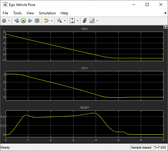

The simulation results are similar to the MATLAB simulation. The ego vehicle has parked at the target pose successfully without collisions with any obstacles.
Conclusion
This example shows how to design two nonlinear MPC controllers, path planner and driving controller, for parallel parking. Both NLMPC controllers navigate the ego vehicle to the target parking spot without colliding with any obstacles.
% Enable message display
mpcverbosity('on');

% Close Simulink model
bdclose(mdl)

% Close animation plots
f = findobj('Name','Automated Parallel Parking');
close(f)
References
[1] Schulman, John, Yan Duan, Jonathan Ho, Alex Lee, Ibrahim Awwal, Henry Bradlow, Jia Pan, Sachin Patil, Ken Goldberg, and Pieter Abbeel. ‘Motion Planning with Sequential Convex Optimization and Convex Collision Checking’. The International Journal of Robotics Research 33, no. 9 (August 2014): 1251–70. https://doi.org/10.1177/0278364914528132.