Test MPC Controller Robustness Using MPC Designer
This example shows how to test the sensitivity of your model predictive controller to prediction errors using simulations, within MPC Designer.
It is good practice to test the robustness of your controller to prediction errors. Classical phase and gain margins are one way to quantify robustness for a SISO application. Robust Control Toolbox™ software provides more sophisticated approaches for MIMO systems. It can also be helpful to assess robustness by running simulations with selected model mismatches and disturbances.
Define Plant Model
For this example, use the CSTR model described in CSTR Model and used in Design Controller Using MPC Designer.
In this model, the first two state variables are the concentration of reagent (here referred to as CA and measured in kmol/m3) and the temperature of the reactor (here referred to as T, measured in K), while the first two inputs are the coolant temperature (Tc, measured in K, used to control the plant), and the inflow feed reagent concentration CAf measured in kmol/m3, (often considered as unmeasured disturbance).
Create a state-space model of the CSTR system.
A = [   -5  -0.3427;
     47.68    2.785];
B = [    0   1
       0.3   0];
C = flipud(eye(2));
D = zeros(2);
CSTR = ss(A,B,C,D);
Specify Signal Names and Types
Assume that the feed flow reagent concentration CAf is an unmeasured disturbance and the reagent concentration CA is an unmeasured output.
CSTR.InputName = {'T_c','C_A_f'};
CSTR.OutputName = {'T','C_A'};
CSTR.StateName = {'C_A','T'};
CSTR = setmpcsignals(CSTR,'MV',1,'UD',2,'MO',1,'UO',2);
Open MPC Designer, and import the plant model.
mpcDesigner(CSTR)
The app imports the plant model and adds it to the Data Browser. It also creates a default controller and a default simulation scenario.
Design Controller
Typically, you would design your controller by specifying scaling factors, defining constraints, and adjusting tuning weights. For this example, modify the controller sample time, and keep the other controller settings at their default values.
In MPC Designer, on the Tuning tab, in the
Horizon section, specify a Sample time of
0.25 seconds.
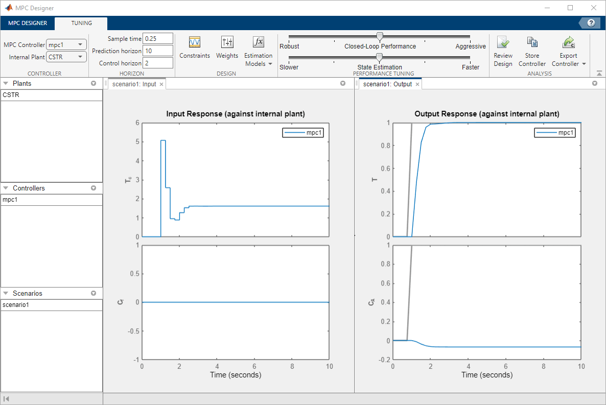
The Input Response and Output Response plots update to reflect the new sample time.
Configure Simulation Scenario
To test controller setpoint tracking and unmeasured disturbance rejection, modify the default simulation scenario.
In the Scenarios section in the lower left part of MPC
Designer, right-click scenario1, and select
Edit.
In the Simulation Scenario dialog box, keep a Simulation duration
of 10 seconds.
In the Reference Signals table, keep the default Ref of
T setpoint configuration, which simulates a unit-step change in the reactor
temperature.
To hold the concentration setpoint at its nominal value, in the second row, in the
Signal drop-down list, select
Constant.
Simulate a unit-step unmeasured disturbance at a time of 5 seconds. In the
Unmeasured Disturbances table, in the Signal
drop-down list, select Step, and specify a
Time of 5.

Click OK.

The app runs the simulation scenario, and updates the response plots to reflect the new simulation settings, so the closed loop responses to the input steps in the measured and unmeasured inputs are shown. For this scenario, the internal model of the controller is used in the simulation. Therefore, the simulation results represent the controller performance when there are no prediction errors.
Define Perturbed Plant Models
Suppose that you want to test the sensitivity of your controller to plant changes that
modify the effect of the coolant temperature on the reactor temperature. You can simulate
such changes by perturbing element B(2,1) of the CSTR input-to-state
matrix. For this example, specify a perturbation amounting to 66% of the nominal value of
B(2,1).
In the MATLAB® Command Window, specify a perturbation matrix.
dB = [0 0; 0.2 0];
Create the two perturbed plant models.
perturbUp = CSTR;
perturbUp.B = perturbUp.B + dB;

perturbDown = CSTR;
perturbDown.B = perturbDown.B - dB;
Examine Step Responses of Perturbed Plants
To examine the effects of the plant perturbations, plot the plant step responses.
step(CSTR,perturbUp,perturbDown)
legend('CSTR','peturbUp','perturbDown')
To set the vertical axes limits from 0 to 1.5
for the top plots and from -0.1 to 0 for the bottom
plots, right-click on the axis, select Properties..., and place the
appropriate limits in the Y-Limits area of the
Limits tab.
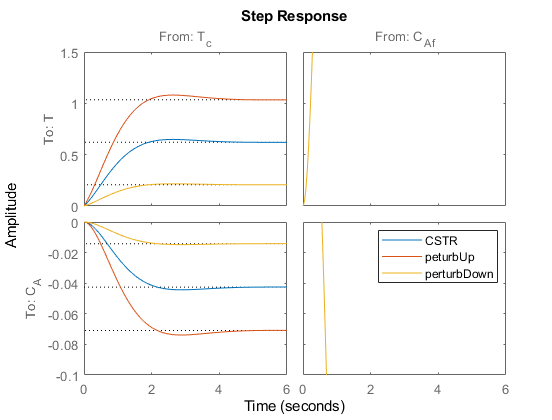
Perturbing element B(2,1) of the CSTR plant changes the magnitude
of the response from the coolant temperature, Tc
to both the reactor temperature, T, and reactor reagent concentration,
CA outputs.
Import Perturbed Plants
In MPC Designer, on the MPC Designer tab, in the Import section, click Import Plant.
In the Import Plant Model dialog box, select the perturbUp and
perturbDown models.

Click Import.
The app imports the models and adds them to the Data Browser.
Define Perturbed Plant Simulation Scenarios
Create two simulation scenarios that use the perturbed plant models.
In the Scenarios section in the lower left part of MPC
Designer, click scenario1, and rename it
accurate.
Right-click accurate, and click Copy.
Rename accurate_Copy to errorUp.
Right-click errorUp, and select Edit.
In the Simulation Scenario dialog box, in the Plant used in
simulation drop-down list, select
perturbUp.
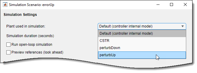
Click OK.
Repeat this process for the second perturbed plant.
Copy the accurate scenario and rename it to
errorDown.
Edit errorDown, selecting the
perturbDown plant.

Examine errorUp Simulation Response
On the MPC Designer tab, in the Scenario section, click Plot Scenario > errorUp.

The app creates the errorUp: Input and errorUp: Output tabs, and displays the simulation response.
To view the accurate and errorUp responses
side-by-side, drag the accurate: Output tab into the left plot
panel.
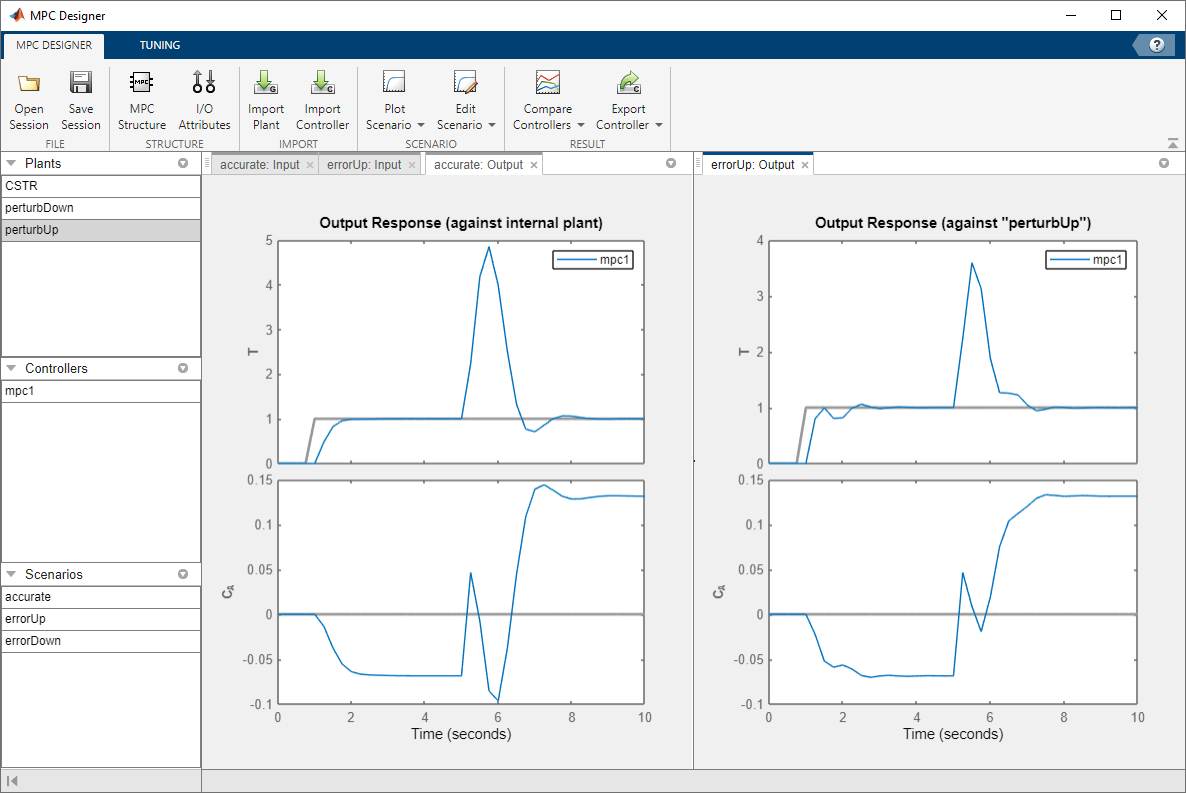
The perturbation creates a plant, perturbUp, that responds slightly
faster to manipulated variable changes than the controller predicts. On the
errorUp: Output tab, in the Output Response
plot, the T setpoint step response oscillates more before settling.
Although this response is, as expected, worse than the response of the
accurate simulation, it is still acceptable. The faster plant
response leads to a smaller peak error in the response to the unmeasured disturbance.
Overall, the controller is able to control the perturbUp plant
successfully despite the internal model prediction error.
Examine errorDown Simulation Response
On the MPC Designer tab, in the Scenario section, click Plot Scenario > errorDown.
The app creates the errorDown: Input and errorDown: Output tabs, and displays the simulation response.
To view the accurate and errorDown responses
side-by-side, click the accurate: Output tab in the left display
panel.

The perturbation creates a plant, perturbDown, that responds slower
to manipulated variable changes than the controller predicts. On the errorDown:
Output tab, in the Output Response plot, the setpoint
tracking and disturbance rejection are worse than for the unperturbed plant.
Depending on the application requirements and the real-world potential for such plant
changes, the degraded response for the perturbDown plant might require
modifications to the controller design.