Tuning MPC Controller Weights at Run-Time
This example shows how to vary the weights on outputs, inputs, and ECR slack variable for soft constraints at run-rime, using either Simulink® or mpcmove.
The weights specified in the MPC object are overridden by the weights supplied to the MPC Controller block. If a weight signal is not connected to the MPC Controller block, then the corresponding weight is the one specified in the MPC object.
Define Plant Model
Define a multivariable discrete-time linear system with no direct I/O feedthrough, and assume input #4 is a measured disturbance and output #4 is unmeasured.
Ts = 0.1; % sampling time
plant = tf({1,[1 1],5,2;3,[1 5],1,0;0,0,1,[1 1];2,[1 -1],0,0}, ...
    {[1 1 1],[1 3 4 5],[1 10],[1 5];
      [1 1],[1 2],[1 2 8],[1 1];
      [1 2 1],[1 3 1 1],[1 1],[1 2];
      [1 1],[1 3 10 10],[1 10],[1 1]});
plant = c2d(ss(plant),Ts);
plant.D = 0;

% display size of the plant.
size(plant)
State-space model with 4 outputs, 4 inputs, and 17 states.
Design MPC Controller
Specify input and output signal types.
plant = setmpcsignals(plant,'MD',4,'UO',4);
% Create the controller object with sampling period, prediction and control
% horizons:
p = 20;                                     % Prediction horizon
m = 3;                                      % Control horizon
mpcobj = mpc(plant,Ts,p,m);

% note that default weights are assumed on inputs, input rates, and outputs
-->Assuming unspecified input signals are manipulated variables.
-->Assuming unspecified output signals are measured outputs.
-->"Weights.ManipulatedVariables" is empty. Assuming default 0.00000.
-->"Weights.ManipulatedVariablesRate" is empty. Assuming default 0.10000.
-->"Weights.OutputVariables" is empty. Assuming default 1.00000.
   for output(s) y1 y2 y3 and zero weight for output(s) y4
Specify MV constraints.
mpcobj.MV(1).Min = -6;
mpcobj.MV(1).Max = 6;
mpcobj.MV(2).Min = -6;
mpcobj.MV(2).Max = 6;
mpcobj.MV(3).Min = -6;
mpcobj.MV(3).Max = 6;
Define Time-Varying Signals Using Structure Format
Define reference signal.
Tstop = 10;
ref = [1 0 3 1];
r = struct('time',(0:Ts:Tstop)');
N = numel(r.time);
r.signals.values=ones(N,1)*ref;
Define measured disturbance.
v = 0.5;
OV weights are linearly increasing with time, except for output #2 that is not weighted.
ywt.time = r.time;
ywt.signals.values = (1:N)'*[.1 0 .1 .1];
MV rate weights are decreasing linearly with time.
duwt.time = r.time;
duwt.signals.values = (1-(1:N)/2/N)'*[.1 .1 .1];
ECR weight increases exponentially with time.
ECRwt.time = r.time;
ECRwt.signals.values = 10.^(2+(1:N)'/N);
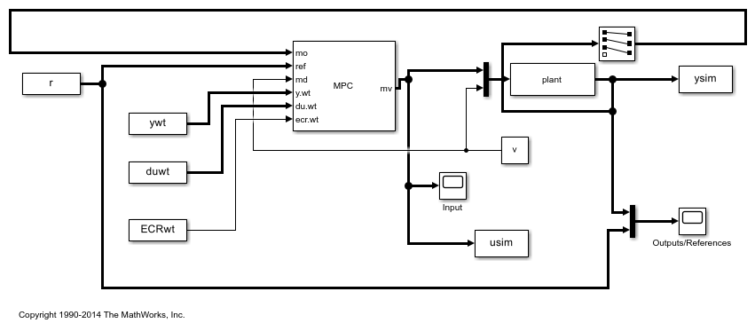
Simulate Using Simulink
Start simulation.
mdl = 'mpc_onlinetuning';
open_system(mdl);                   % Open Simulink(R) Model
sim(mdl);                           % Start Simulation
-->Integrator added as output disturbance model for measured output #1.
-->Integrator added as output disturbance model for measured output #2.
-->Integrator added as output disturbance model for measured output #3.
-->"Model.Noise" is empty. Assuming white noise on each measured output.
Simulate Using MPCMOVE Command
Define real plant and MPC state object.
[A,B,C,D] = ssdata(plant);
x = zeros(size(plant.B,1),1);   % Initial state of the plant
xmpc = mpcstate(mpcobj);        % Handle to state of the MPC controller
Store the closed-loop MPC trajectories in arrays YY,UU,XX.
YY = []; UU = []; XX = [];
Use mpcmoveopt object to provide weights at run-time.
options = mpcmoveopt;
Start simulation.
for t = 0:N-1,
    % Store states
    XX = [XX,x]; %#ok<*AGROW>
    % Compute and store plant output (no feedthrough from MV to Y)
    y = C*x+D(:,4)*v;
    YY = [YY;y'];
    % Obtain reference signal
    ref = r.signals.values(t+1,:)';
    % Update |mpcmoveopt| object with run-time weights
    options.MVRateWeight = duwt.signals.values(t+1,:);
    options.OutputWeight = ywt.signals.values(t+1,:);
    options.ECRWeight = ECRwt.signals.values(t+1,:);
    % Compute and sore control action
    u = mpcmove(mpcobj,xmpc,y(1:3),ref,v,options);
    UU = [UU;u'];
    % Update plant states
    x = A*x + B(:,1:3)*u + B(:,4)*v;
end
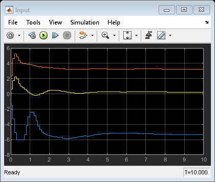
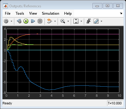
Plot and Compare Simulation Results.
figure(1);
clf;
subplot(121)
plot(0:Ts:Tstop,[YY ysim])
grid
title('output')
subplot(122)
plot(0:Ts:Tstop,[UU usim])
grid
title('input')

Compare input and output signals.
norm(UU-usim)
norm(YY-ysim)

% results are identical except for numerical errors.
ans =

   5.9355e-11


ans =

   1.2495e-11
bdclose(mdl);