Vary Input and Output Bounds at Run Time
This example shows how to vary input and output saturation limits in real-time control. For both command-line and Simulink® simulations, you specify updated input and output constraints at each control interval. The MPC controller then keeps the input and output signals within their specified bounds.
For more information on updating linear constraints at run time, see Update Constraints at Run Time.
Create Plant Model and MPC Controller
Define a SISO discrete-time plant with sample time Ts.
Ts = 0.1;
plant = c2d(tf(1,[1 .8 3]),Ts);
[A,B,C,D] = ssdata(plant);
Create an MPC controller with specified prediction horizon, p, control horizon, c, and sample time, Ts. Use plant as the internal prediction model.
p = 10;
m = 4;
mpcobj = mpc(plant,Ts,p,m);
-->"Weights.ManipulatedVariables" is empty. Assuming default 0.00000.
-->"Weights.ManipulatedVariablesRate" is empty. Assuming default 0.10000.
-->"Weights.OutputVariables" is empty. Assuming default 1.00000.
Specify controller tuning weights.
mpcobj.Weights.MV = 0;
mpcobj.Weights.MVrate = 0.5;
mpcobj.Weights.OV = 1;
For this example, the upper and lower bounds on the manipulated variable, and the upper bound on the output variable are varied at run time. To do so, you must first define initial dummy finite values for these constraints in the MPC controller object. Specify values for MV.Min, MV.Max, and OV.Max.
At run time, these constraints are changed using an mpcmoveopt object at the command line or corresponding input signals to the MPC Controller block.
mpcobj.MV.Min = 1;
mpcobj.MV.Max = 1;
mpcobj.OV.Max = 1;
Simulate Model Using Simulink
Open Simulink model.
mdl = 'mpc_varbounds';
open_system(mdl)
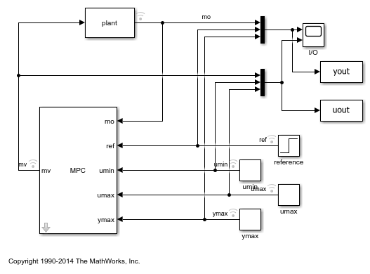
In this model, the input minimum and maximum constraint ports (umin and umax) and the output maximum constraint port (ymax)of the MPC Controller block are enabled. Because the minimum output bound is unconstrained, the ymin input port is disabled.
Configure the output setpoint, ref, and simulation duration, Tsim.
ref = 1;
Tsim = 20;
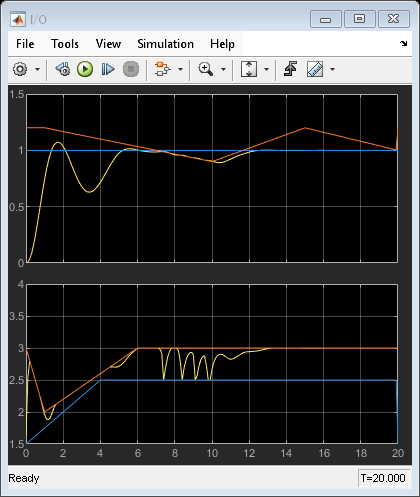
Run the simulation, and view the input and output responses in the I/O scope.
sim(mdl)
open_system([mdl '/I//O'])
-->Converting the "Model.Plant" property to state-space.
-->Integrator added as output disturbance model for measured output #1.
-->"Model.Noise" is empty. Assuming white noise on each measured output.
Simulate Model at Command Line
Specify the initial state of the plant and controller.
x = zeros(size(B,1),1);
xmpc = mpcstate(mpcobj);
Store the closed-loop output, manipulated variable, and state trajectories of the MPC controller in arrays YY, UU, and XX, respectively.
YY = [];
UU = [];
XX = [];
Create an mpcmoveopt object for specifying the run-time bound values.
options = mpcmoveopt;
Run the simulation loop.
for t = 0:round(Tsim/Ts)
    % Store the plant state.
    XX = [XX; x];

    % Compute and store the plant output. There is no direct feedthrough
    % from the input to the output.
    y = C*x;
    YY = [YY; y'];

    % Get the reference signal value from the data output by the Simulink
    % simulation.
    ref = yout.Data(t+1,2);

    % Update the input and output bounds. For consistency, use the
    % constraint values output by the Simulink simulation.
    options.MVMin = uout.Data(t+1,2);
    options.MVMax = uout.Data(t+1,3);
    options.OutputMax = yout.Data(t+1,3);

    % Compute the MPC control action.
    u = mpcmove(mpcobj,xmpc,y,ref,[],options);

    % Update the plant state and store the input signal value.
    x = A*x + B*u;
    UU = [UU; u'];
end
Compare Simulation Results
Plot the input and output signals from both the Simulink and command-line simulations along with the changing input and output bounds.
figure
subplot(1,2,1)
plot(0:Ts:Tsim,[UU uout.Data(:,1) uout.Data(:,2) uout.Data(:,3)])
grid
title('Input')
legend('Command-line input','Simulink input','Lower bound', ...
    'Upper bound','Location','Southeast')
subplot(1,2,2)
plot(0:Ts:Tsim,[YY yout.Data(:,1) yout.Data(:,3)])
grid
title('Output')
legend('Command-line output','Simulink output','Upper bound', ...
    'Location','Southeast')

The results of the command-line and Simulink simulations are the same. The MPC controller keeps the input and output signals within the specified bounds as the constraints change throughout the simulation.
bdclose(mdl)
