Specify Constraints
Input and Output Constraints
By default, when you create a controller object using the mpc command, no constraints exist. To include a constraint, set the appropriate
controller property. The most common MPC constraints are bounds on single inputs or outputs,
however, you can also introduce (and update at run time) mixed input/output linear
constraints (see Constraints on Linear Combinations of Inputs and Outputs, and Update Mixed Input/Output Constraints at Run Time).
The following table summarizes the controller properties used to define bounds on specific variables. (MV = plant manipulated variable; OV = plant output variable; MV increment = u(k) – u(k – 1).
| Constraint | Controller Property | Constraint Softening |
|---|---|---|
| Lower bound on ith MV | MV(i).Min > -Inf | MV(i).MinECR > 0 |
| Upper bound on ith MV | MV(i).Max < Inf | MV(i).MaxECR > 0 |
| Lower bound on ith OV | OV(i).Min > -Inf | OV(i).MinECR > 0 |
| Upper bound on ith OV | OV(i).Max < Inf | OV(i).MaxECR > 0 |
| Lower bound on ith MV increment | MV(i).RateMin > -Inf | MV(i).RateMinECR > 0 |
| Upper bound on ith MV increment | MV(i).RateMax < Inf | MV(i).RateMaxECR > 0 |
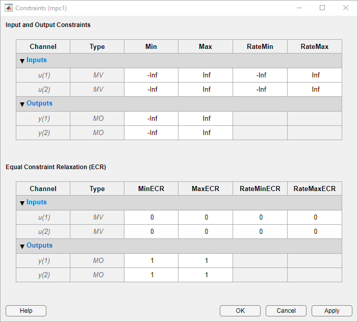
To set the controller constraint properties using the MPC Designer app, in
the Tuning tab, click Constraints
![]() . In the Constraints dialog box, specify the constraint
values.
. In the Constraints dialog box, specify the constraint
values.
See Constraints for the equations describing the corresponding constraints, where:
corresponds to the i-th element of the
MinECRvector stored in the j-th element of theOutputVariablesproperty of anmpcobject.corresponds to the i-th element of the
MaxECRvector stored in the j-th element of theOutputVariablesproperty of anmpcobject.corresponds to the i-th element of the
MinECRvector stored in the j-th element of theManipulatedVariablesproperty of anmpcobject.corresponds to the i-th element of the
MaxECRvector stored in the j-th element of theManipulatedVariablesproperty of anmpcobject.corresponds to the i-th element of the
RateMinECRvector stored in the j-th element of theManipulatedVariablesproperty of anmpcobject.corresponds to the i-th element of the
RateMaxECRvector stored in the j-th element of theManipulatedVariablesproperty of anmpcobject.
For more information on updating constraints at run time, see Update Constraints at Run Time.
Tips
For MV bounds:
Include known physical limits on the plant MVs as hard MV bounds.
Include MV increment bounds when there is a known physical limit on the rate of change, or your application requires you to prevent large increments for some other reason.
Do not include both hard MV bounds and hard MV increment bounds on the same MV, as they can conflict. If both types of bounds are important, soften one.
For OV bounds:
Do not include OV bounds unless they are essential to your application. As an alternative to setting an OV bound, you can define an OV reference and set its cost function weight to keep the OV close to its setpoint.
All OV constraints should be softened.
Consider leaving the OV unconstrained for some prediction horizon steps. See Setting Time-Varying Weights and Constraints with MPC Designer.
Consider a time-varying OV constraint that is easy to satisfy early in the horizon, gradually tapering to a more strict constraint. See Setting Time-Varying Weights and Constraints with MPC Designer.
Do not include OV constraints that are impossible to satisfy. Even if soft, such constraints can cause unexpected controller behavior. For example, consider a SISO plant with five sampling periods of delay. An OV constraint before the sixth prediction horizon step is, in general, impossible to satisfy. You can use the
reviewcommand to check for such impossible constraints, and use a time-varying OV bound instead. See Setting Time-Varying Weights and Constraints with MPC Designer.
Constraint Softening
Hard constraints are constraints that the quadratic programming (QP) solution must satisfy. If it is mathematically impossible to satisfy a hard constraint at a given control interval, k, the QP is infeasible. In this case, the controller returns an error status, and sets the manipulated variables (MVs) to u(k) = u(k–1), that is, no change. If the condition leading to infeasibility is not resolved, infeasibility can continue indefinitely, leading to a loss of control.
Disturbances and prediction errors are inevitable in practice. Therefore, a constraint violation could occur in the plant even though the controller predicts otherwise. A feasible QP solution does not guarantee that all hard constraints will be satisfied when the optimal MV is used in the plant.
If the only constraints in your application are bounds on MVs, the MV bounds can be hard constraints, as they are by default. MV bounds alone cannot cause infeasibility. The same is true when the only constraints are on MV increments.
However, a hard MV bound with a hard MV increment constraint can lead to infeasibility. For example, an upset or operation under manual control could cause the actual MV used in the plant to exceed the specified bound during interval k–1. If the controller is in automatic during interval k, it must return the MV to a value within the hard bound. If the MV exceeds the bound by too much, the hard increment constraint can make correcting the bound violation in the next interval impossible.
If the plant is subject to disturbances and there are either hard output constraints or hard mixed input-output constraints, then QP infeasibility is a distinct possibility.
All Model Predictive Control Toolbox™ constraints (except slack variable nonnegativity) can be soft. When a constraint is soft, the controller can deem an MV optimal even though it predicts a violation of that constraint. If all plant output, MV increment, and custom constraints are soft (as they are by default), QP infeasibility does not occur. However, controller performance can be substandard.
To soften a constraint, set the corresponding equal concern for relaxation (ECR) value to a positive value (zero implies a hard constraint). The larger the ECR value, the more likely the controller will deem it optimal to violate the constraint in order to satisfy your other performance goals. The Model Predictive Control Toolbox software provides default ECR values but, as for the cost function weights, you might need to tune the ECR values in order to achieve acceptable performance.
To understand how constraint softening works, suppose that your cost function uses , giving both the MV and MV increments zero weight in the cost function. Only the output reference tracking and constraint violation terms are nonzero. In this case, the cost function is:
Suppose that you have also specified hard MV bounds with and . Then these constraints simplify to:
Thus, the dimensionless slack variable for constraint softening, εk, no longer appears in the above equations. You have also specified soft constraints on plant outputs with and .
Now, suppose that a disturbance has pushed a plant output above its specified upper bound, but the QP with hard output constraints would be feasible, that is, all constraint violations could be avoided in the QP solution. The QP involves a tradeoff between output reference tracking and constraint violation. The slack variable, εk, must be nonnegative. Its appearance in the cost function discourages, but does not prevent, an optimal εk > 0. A larger ρε weight, however, increases the likelihood that the optimal εk will be small or zero.
If the optimal εk > 0, at least one of the bound inequalities must be active (at equality). A relatively large makes it easier to satisfy the constraint with a small εk. In that case,
can be larger, without exceeding
Notice that does not set an upper limit on the constraint violation. Rather, it is a tuning factor determining whether a soft constraint is easy or difficult to satisfy.
Tips
Use of dimensionless variables simplifies constraint tuning. Define appropriate scale factors for each plant input and output variable. See Specify Scale Factors.
To indicate the relative magnitude of a tolerable violation, use the ECR parameter associated with each constraint. Rough guidelines are as follows:
0 — No violation allowed (hard constraint)
0.05 — Very small violation allowed (nearly hard)
0.2 — Small violation allowed (quite hard)
1 — average softness
5 — greater-than-average violation allowed (quite soft)
20 — large violation allowed (very soft)
Use the overall constraint softening parameter of the controller (controller object property:
Weights.ECR) to penalize a tolerable soft constraint violation relative to the other cost function terms. Set theWeights.ECRproperty such that the corresponding penalty is 1–2 orders of magnitude greater than the typical sum of the other three cost function terms. If constraint violations seem too large during simulation tests, try increasingWeights.ECRby a factor of 2–5.Be aware, however, that an excessively large
Weights.ECRdistorts MV optimization, leading to inappropriate MV adjustments when constraint violations occur. To check for this, display the cost function value during simulations. If its magnitude increases by more than 2 orders of magnitude when a constraint violation occurs, consider decreasingWeights.ECR.Disturbances and prediction errors can lead to unexpected constraint violations in a real system. Attempting to prevent these violations by making constraints harder often degrades controller performance.