DC Servomotor with Constraint on Unmeasured Output
This example shows how to design a model predictive controller for a DC servomechanism under voltage and shaft torque constraints.
For a similar example that uses explicit MPC, see Explicit MPC Control of DC Servomotor with Constraint on Unmeasured Output. For a related example with this plant, see Design MPC Controller for Position Servomechanism.
Define DC-Servo Motor Model
The mpcmotormodel function returns the plant model needed for the example. The linear open-loop dynamic model is defined in plant. The variable tau is the maximum admissible torque; this is going to be used as an output constraint.
[plant,tau] = mpcmotormodel;
Display basic plant characteristics.
size(plant)
damp(plant)
State-space model with 2 outputs, 1 inputs, and 4 states.

         Pole              Damping       Frequency      Time Constant
                                       (rad/seconds)      (seconds)

  1.52e-15                -1.00e+00       1.52e-15        -6.59e+14
 -7.05e-01 + 7.31e+00i     9.59e-02       7.35e+00         1.42e+00
 -7.05e-01 - 7.31e+00i     9.59e-02       7.35e+00         1.42e+00
 -9.79e+00                 1.00e+00       9.79e+00         1.02e-01
The plant control input is the DC voltage, the four state variables are the angular position and velocities of the load and the motor shaft. The measurable output is the angular position of the load. The second output, torque, is not measurable. For more information, see Design MPC Controller for Position Servomechanism.
Specify input and output signal types for the MPC controller.
plant = setmpcsignals(plant,'MV',1,'MO',1,'UO',2);
Specify MV Constraints
The manipulated variable is constrained between +/- 220 volts. Because the plant inputs and outputs are of different orders of magnitude, you also use scale factors to facilitate MPC tuning. Typical choices of scale factor are the upper/lower limit or the operating range.
MV = struct('Min',-220,'Max',220,'ScaleFactor',440);
Specify OV Constraints
Torque constraints of +|tau| and -|tau| are only imposed during the first three prediction steps. Also specify a scale factor for both outputs (load angle and torque).
OV = struct('Min',{-Inf, [-tau;-tau;-tau;-Inf]}, ...
            'Max',{Inf, [tau;tau;tau;Inf]}, ...
            'ScaleFactor',{2*pi, 2*tau});
Specify Tuning Weights
The control task is to get zero tracking offset for the angular position. Because you only have one manipulated variable, the shaft torque is allowed to float within its constraint by setting its weight to zero.
Weights = struct('MV',0,'MVRate',0.1,'OV',[0.1 0]);
Create MPC Controller
Create an MPC controller with sample time Ts, prediction horizon of 10 steps, and control horizon of 2 steps.
Ts = 0.1;
mpcobj = mpc(plant,Ts,10,2,Weights,MV,OV);
Calculate Closed Loop DC Gain Matrix
Calculate the steady state output sensitivity of the closed loop. A zero value means that the measured plant output can track the desired output reference setpoint.
cloffset(mpcobj)
-->Converting model to discrete time.
   Assuming no disturbance added to measured output #1.
-->"Model.Noise" is empty. Assuming white noise on each measured output.

ans =

   1.1102e-16
Simulate Controller Using sim Function
Use the sim function to simulate the closed-loop control of the linear plant model in MATLAB®.
disp('Now simulating nominal closed-loop behavior');
Tstop = 8;                      % seconds
Tf = round(Tstop/Ts);           % simulation iterations
r = [pi*ones(Tf,1) zeros(Tf,1)];% reference signal
[y1,t1,u1] = sim(mpcobj,Tf,r);
Now simulating nominal closed-loop behavior
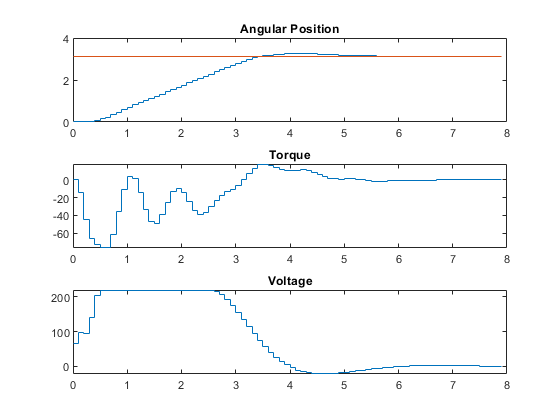
Plot results.
subplot(3,1,1)
stairs(t1,y1(:,1))
hold on
stairs(t1,r(:,1))
hold off
title('Angular Position')

subplot(3,1,2)
stairs(t1,y1(:,2))
title('Torque')

subplot(3,1,3)
stairs(t1,u1)
title('Voltage')
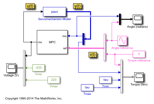
Simulate Using Simulink
Simulate the closed-loop in Simulink®. The MPC Controller block is configured to use mpcobj as its controller.
mdl = 'mpc_motor';
open_system(mdl)
sim(mdl)
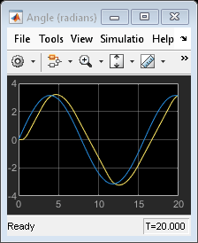
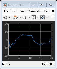
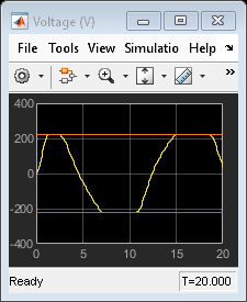
The closed-loop response is identical to the simulation result in MATLAB.
References
[1] A. Bemporad and E. Mosca, "Fulfilling hard constraints in uncertain linear systems by reference managing," Automatica, vol. 34, no. 4, pp. 451-461, 1998.
bdclose(mdl)