Monitor Solution Process with optimplot
This example shows how you can use the optimplot plot function to monitor several aspects of the solution process.
Note: Currently, optimplot is available only for the fmincon solver.
Problem Definition and First Solution
The problem is to minimize the objective function of two variables
in the region , , . Express this problem using optimization variables.
x = optimvar("x",LowerBound=-5);
y = optimvar("y",LowerBound=-5);
prob = optimproblem;
prob.Objective = (x+y)*exp(-y);
prob.Constraints = (y + x^2)^2 + 0.1*y^2 <= 1;
Set an initial point of .
x0.x = 1;
x0.y = -3/2;
Which solver does solve call?
defaultSolver = solvers(prob)
defaultSolver =
"fmincon"
Set fmincon options to use the optimplot plot function, and solve the problem.
opts = optimoptions("fmincon",PlotFcn="optimplot");
[sol,fval,eflag,output] = solve(prob,x0,Options=opts);
Solving problem using fmincon.
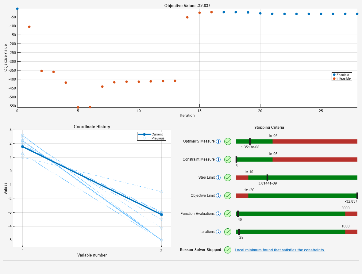
Local minimum found that satisfies the constraints.

Optimization completed because the objective function is non-decreasing in
feasible directions, to within the value of the optimality tolerance,
and constraints are satisfied to within the value of the constraint tolerance.

<stopping criteria details>
Plot Details
Examine each section of the plot, beginning with the top section.
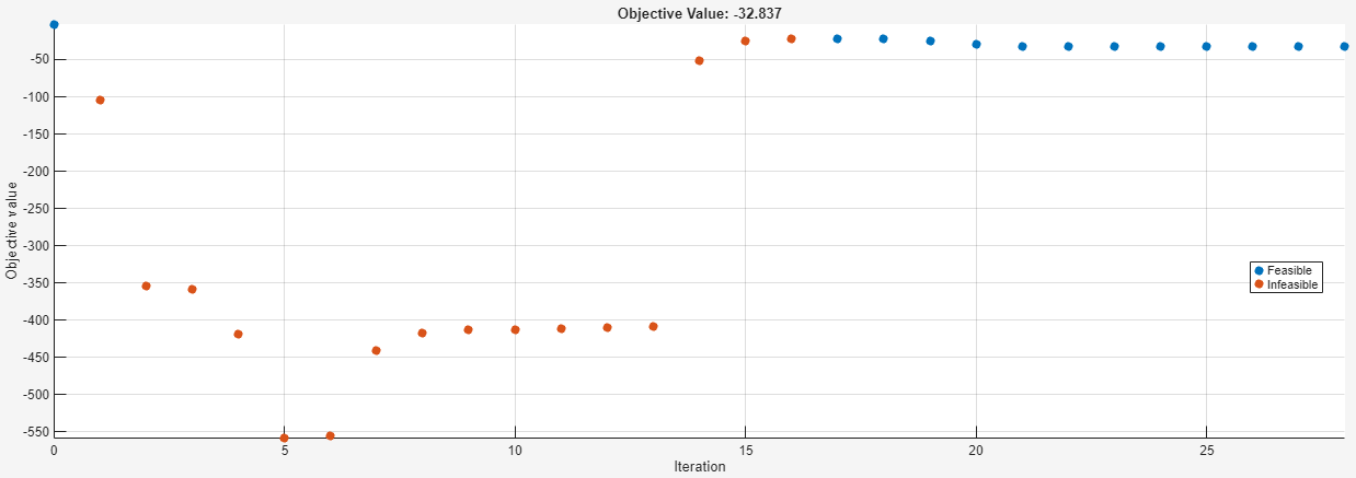
The plot shows that the initial point (at the upper left) is feasible, because it is plotted as a blue dot. "Feasible" means the point satisfies all constraints, "infeasible" means a point does not satisfy at least one constraint. The next several points are red dots, which means they are infeasible. The right portion of the plot contains all blue dots, indicating feasible iterations.
Next, examine the variable plot, which is the lower-left section.
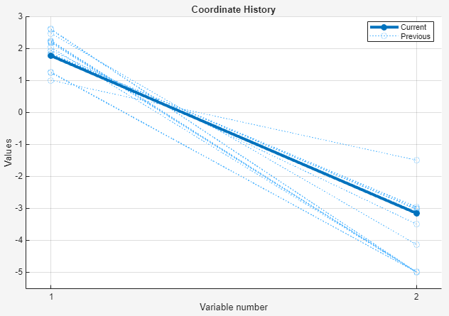
The final point is plotted as a bold line. The intermediate iterations are plotted as fainter dotted lines.
Finally, examine the lower-right section, which contains the stopping criteria.
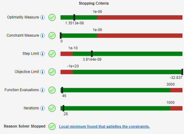
This section provides the following information:
Optimality Measure --- This bar shows that the first-order optimality measure is satisfied. The marker is in the green region, and the value is less than the
OptimalityTolerancevalue of 1e–6. This tolerance stopped the solver.Constraint Measure --- This bar shows that the constraints are all satisfied to within the value of the
ConstraintTolerance, 1e–6. This tolerance is not an actual stopping criterion. Instead, solvers attempt to continue when the constraints are not satisfied.Step Limit --- This bar shows that the solver was not stopped by the
StepTolerancetolerance.Objective Limit --- This bar shows that the solver was not stopped by the
ObjectiveLimittolerance.Function Evaluations --- This bar shows that the solver was not stopped by the
MaxFunctionEvaluationstolerance.Iterations --- This bar shows that the solver was not stopped by the
MaxIterationstolerance.
Note that a solver can use relative or scaled values of stopping criteria. For details, see Tolerance Details.
The three sections of the plot are synchronized. When you click a point in the top section, all three sections display values associated with that point. Click the fifth iteration point.
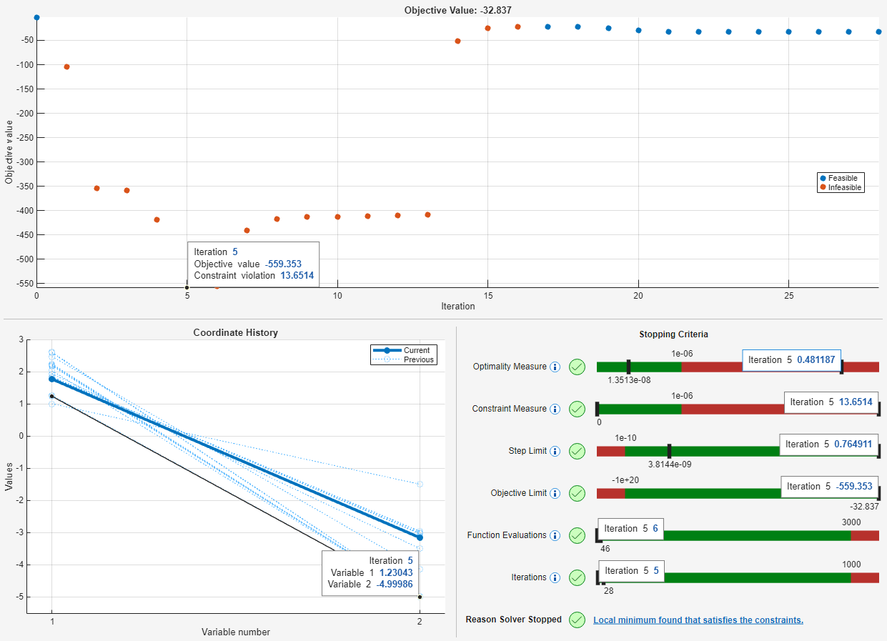
The fifth iteration point has the lowest objective function value. However, the point is not feasible. As shown in the top section, the point is plotted in red, and has a constraint violation of over 13. The Constraint Measure bar in the Stopping Criteria section shows the same value for the violation, which also indicates that the point is infeasible. To remove the displayed values for the fifth iteration, click the point again.
Dynamic Plotting Range
You might have noticed that the initial point was not visible during the early iterations while the solver was running. Below is a close-up of the plot function, paused after the seventh iteration.
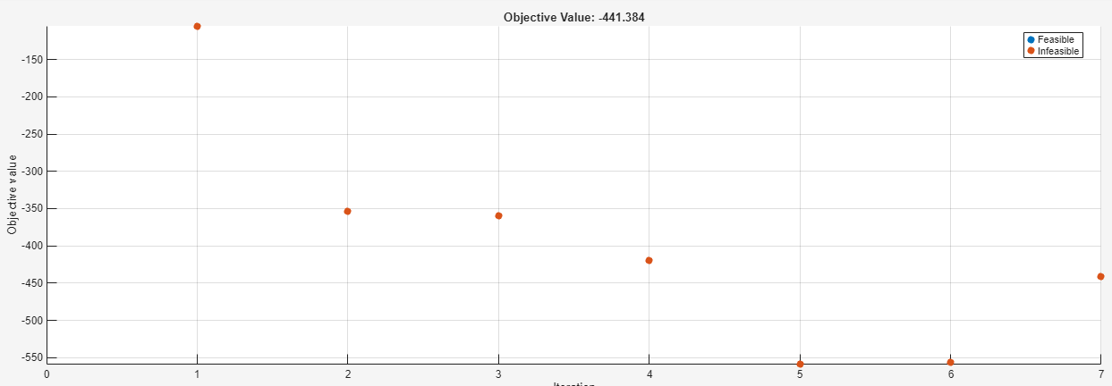
The point for iteration 0 is not plotted because it is outside the plot range. The optimplot plot function attempts to show relevant ranges as the iterations proceed, so that you can observe convergence more easily.
Search for Better Solution
The bottom of the Stopping Criteria section shows the reason the solver stopped, and provides a link for more information.
![]()
Click the link, and you get the following information and link.
![]()
Click the link When the Solver Succeeds. In the resulting documentation page, the first suggestion is to change the initial point. So, search for a better solution by changing the initial point.
x0.x = -1;
x0.y = -1;
[sol2,fval2,eflag2,output2] = solve(prob,x0,Options=opts);
Solving problem using fmincon.
Local minimum found that satisfies the constraints.

Optimization completed because the objective function is non-decreasing in
feasible directions, to within the value of the optimality tolerance,
and constraints are satisfied to within the value of the constraint tolerance.

<stopping criteria details>
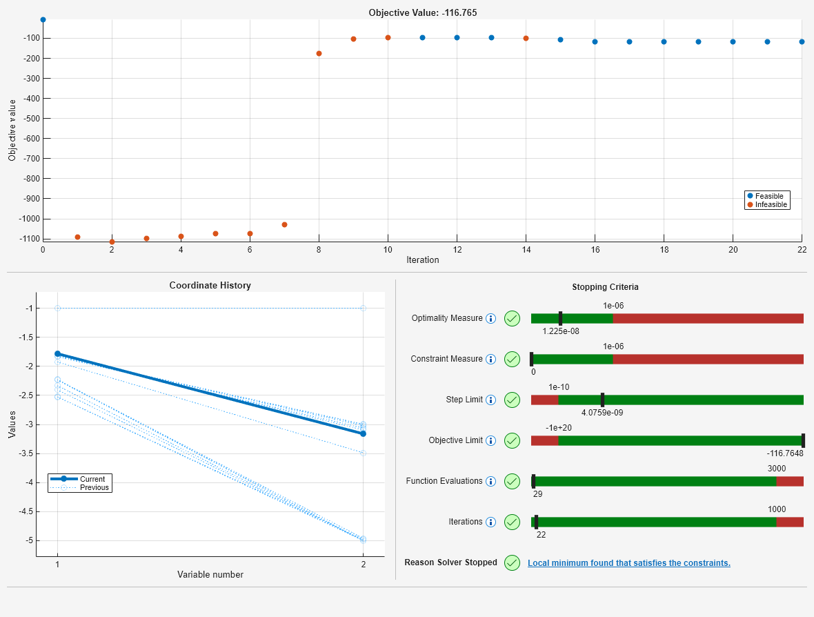
This time, the plot shows that fmincon reaches an objective function value of , which is better (lower) than the value at the first solution, .
Conclusions
The optimplot plot function shows many of the statistics associated with solver iterations. In one plot, you can view the feasibility of the iterative points, the various measures used to stop the iterations, and the coordinates of the iterative points, with the later points plotted in bold. However, the optimplot plot function does not guarantee that the displayed solutions are global solutions. The first solution in this example is a local solution, but not a global solution. Interpreting the results appropriately still requires good judgment.