phased.MatchedFilter

Matched filter

Description

The phased.MatchedFilter System object™ implements matched filtering of an input signal. To compute the matched filtered signal:

1. Create the phased.MatchedFilter object and set its properties.

2. Call the object with arguments, as if it were a function.

To learn more about how System objects work, see What Are System Objects?

Creation

Syntax

mfilter = phased.MatchedFilter

mfilter = phased.MatchedFilter(Name=Value)

Description

mfilter = phased.MatchedFilter creates a matched filter System object, mfilter. The object performs matched filtering on the input data.

mfilter = phased.MatchedFilter(Name=Value) creates a matched filter object, mfilter, with each specified property Name set to the specified Value. You can specify additional name-value pair arguments in any order as (Name1=Value1, ..., NameN=ValueN).

Properties

Unless otherwise indicated, properties are nontunable, which means you cannot change their values after calling the object. Objects lock when you call them, and the release function unlocks them.

If a property is tunable, you can change its value at any time.

For more information on changing property values, see System Design in MATLAB Using System Objects.

CoefficientsSource — Source of matched filter coefficients

'Property' (default) | Coefficients

Source of matched filter coefficients, specified as 'Property' or Coefficients.

'Property'	Use the Coefficients property to specify the matched coefficients.
'Input port'	Specify the coefficients using an input argument when calling the matched filter.

Example: 'Input port'

Data Types: char | string

Coefficients — Matched filter coefficients

[1;1] (default) | complex-valued column vector

Matched filter coefficients, specified as a complex-valued column vector. Many waveform System objects have an object function such as getMatchedFilter which returns matched filter coefficients derived from the waveform.

Example: [1;1]

Tunable: Yes

Dependencies

To enable this property, set the CoefficientsSource property to 'Property'.

Data Types: double

SpectrumWindow — Spectrum weighting window type

'None' (default) | 'Hamming' | 'Chebyshev' | 'Hann' | 'Kaiser' | 'Taylor' | 'Custom'

Spectrum weighting window type, specified as 'None', 'Hamming', 'Chebyshev', 'Hann', 'Kaiser', 'Taylor', or 'Custom'. The object computes the window length internally, to match the FFT length. For example, spectrum weighting is often used with linear FM waveform to reduce sidelobes in the time domain. Available spectrum weighting functions are:

Spectrum window functions

Chebyshev	chebwin
Hamming	hamming
Hann	barthannwin
Kaiser	kaiserwin
Taylor	taylorwin

Example: 'Taylor'

Data Types: char | string

CustomSpectrumWindow — User-defined window for spectrum weighting

@hamming (default) | function handle | cell array

User-defined window for spectrum weighting, specified as a function handle or a cell array.

If CustomSpectrumWindow is a function handle, the specified function takes the window length as the input and generates appropriate window coefficients.

If CustomSpectrumWindow is a cell array, then the first cell must be a function handle. The specified function takes the window length as the first input argument, with other additional input arguments if necessary, and generates appropriate window coefficients. The remaining entries in the cell array are the additional input arguments to the function, if any.

Example: @kaiser

Dependencies

To enable this property, the SpectrumWindow property to 'Custom'.

Data Types: function_handle | cell

SpectrumRange — Spectrum window coverage region

[0 1e5] (default) | 1-by-2 real-valued vector

Spectrum window coverage region, specified as a 1-by-2 real-valued vector in the form of [StartFrequency EndFrequency]. This property defines the spectrum region on to which the spectrum window is applied.

Note that both StartFrequency and EndFrequency are measured in baseband. That is, they are within [-Fs/2  Fs/2], where Fs is the sample rate that you specify in the SampleRate property. StartFrequency cannot be greater than EndFrequency. Units are in Hz.

Example: [1e4 2e4]

Dependencies

To enable this property, set the SpectrumWindow property to a value other than 'None'.

Data Types: double

SampleRate — Coefficient sample rate

1e6 (default) | positive scalar

Matched filter coefficients sample rate, specified as a positive scalar. Units are in Hz.

Example: 1e6

Dependencies

To enable this property, set the SpectrumWindow property to a value other than 'None'.

Data Types: double

SidelobeAttenuation — Window sidelobe attenuation level

30 (default) | scalar

Window sidelobe attenuation level, specified as a scalar. This property applies to Chebyshev or Taylor windows. Units are in dB.

Example: 30

Dependencies

To enable this property, set the SpectrumWindow property to 'Chebyshev' or 'Taylor'.

Data Types: char | string

Beta — Kaiser window parameter

0.5 (default) | nonnegative scalar

Kaiser window parameter, specified as a nonnegative scalar. This property affects the Kaiser window sidelobe attenuation. Please refer to the kaiser function for more details.

Example: 0.76

Dependencies

To enable this property, set the SpectrumWindow property to 'Kaiser'.

Data Types: double

Nbar — Number of nearly-constant sidelobes in Taylor window

4 (default) | positive integer

Number of nearly-constant sidelobes adjacent to the mainlobe in a Taylor window, specified as a positive integer.

Example: 6

Dependencies

To enable this property, set the SpectrumWindow property to 'Tayler'.

Data Types: double

GainOutputPort — Output gain

false (default) | true

Set this property to true to output the matched filter gain from the matched filter. If you do not want to obtain the matched filter gain, set this property to false.

Example: true

Data Types: logical

MaximumNumInputSamplesSource — Maximum number of input samples source

'Auto' (default) | 'Property'

Source of maximum number of samples of the input signal, specified as 'Auto' or 'Property'. When you set this property to 'Auto', the matched filter automatically allocates the memory to buffer the first input signal. When you set this property to 'Property', the maximum number of samples in the input signal is specified via MaximumNumInputSamples property. An input signal that is longer than the allocated buffer is truncated.

Example: 'Property'

Data Types: char | string

MaximumNumInputSamples — Maximum number of samples in input signal

100 (default) | positive integer

Maximum number of samples in the input signal, specified as a positive integer. The input signal is the first input, X, and the number of samples is number of rows in X.

Example: 200

Dependencies

To enable this property, set the MaximumNumInputSamplesSource property to 'Property'.

Data Types: double

Usage

Syntax

Y = mfilter(X)

Y = mfilter(X,COEFF)

[Y,GAIN] = mfilter(___)

Description

Y = mfilter(X) applies matched filtering to the input X and returns the filtered result in Y. The filter is applied along the first dimension of X. Y and X have the same dimensions. Any initial transient is removed from the filtered result.

The size of the first dimension of the input matrix can vary to simulate a changing signal length. A size change can occur, for example, in the case of a pulse waveform with variable pulse repetition frequency.

Y = mfilter(X,COEFF) uses the input COEFF as matched filter coefficients. To use this syntax, set the CoefficientsSource property to 'Input port'.

[Y,GAIN] = mfilter(___) also returns the matched filter GAIN. To use this syntax, set the GainOutputPort property to true.

Input Arguments

X — Filter input

M-length complex-valued vector | M-by-N complex-valued matrix

Filter input, specified as an M-length complex-valued vector or M-by-N complex-valued matrix. The filter is applied along the first dimension.

Data Types: double
Complex Number Support: Yes

COEFF — Matched filter coefficients

complex-valued column vector

Matched filter coefficients, specified as a complex-valued column vector. Many waveform System objects have an object function such as getMatchedFilter which returns matched filter coefficients derived from the waveform.

Dependencies

To enable this argument, set the CoefficientsSource property to 'Input port'.

Data Types: double
Complex Number Support: Yes

Output Arguments

Y — Matched-filter output

M-length complex-valued vector | M-by-N complex-valued matrix

Filter output, returned as an M-length complex-valued vector or M-by-N complex-valued matrix. The size of Y is the same as the size of X.

The matched filter is only applied along the first dimension of X.

Data Types: double
Complex Number Support: Yes

GAIN — Matched filter gain

scalar

Matched filter gain, returned as a scalar.

Dependencies

To enable this output, set the GainOutputPort property to true.

Data Types: double

Object Functions

To use an object function, specify the System object as the first input argument. For example, to release system resources of a System object named obj, use this syntax:

release(obj)

Common to All System Objects

step	Run System object algorithm
release	Release resources and allow changes to System object property values and input characteristics
reset	Reset internal states of System object

Examples

Matched Filter for Linear FM Waveform

Create a linear FM waveform with a pulse repetition frequency of 5kH. Apply a matched filter derived from the waveform.

waveform = phased.LinearFMWaveform('PulseWidth',1e-4, ...
    'PRF',5e3);
x = waveform();
mfilter = phased.MatchedFilter( ...
    'Coefficients',getMatchedFilter(waveform));
y = mfilter(x);

Plot the real parts of the original waveform and the match-filtered waveform.

subplot(2,1,1)
plot(real(x))
xlabel('Samples')
ylabel('Amplitude')
title('Input Signal')
subplot(2,1,2)
plot(real(y))
xlabel('Samples')
ylabel('Amplitude')
title('Matched Filter Output')

Matched Filter Using Hamming Window

Apply a matched filter, using a Hamming window to do spectrum weighting.

waveform = phased.LinearFMWaveform('PulseWidth',1e-4,'PRF',5e3);
x = waveform();
mfilter = phased.MatchedFilter( ...
    'Coefficients',getMatchedFilter(waveform), ...
	'SpectrumWindow','Hamming');
y = mfilter(x);
subplot(2,1,1)
plot(real(x))
xlabel('Samples')
ylabel('Amplitude')
title('Input Signal')
subplot(2,1,2)
plot(real(y))
xlabel('Samples')
ylabel('Amplitude')
title('Matched Filter Output')

Matched Filter with Custom Window

Apply a matched filter to a signal created from a linear FM waveform. Use a custom Gaussian window for spectrum weighting.

waveform = phased.LinearFMWaveform('PulseWidth',1e-4,'PRF',5e3);
x = waveform();
mfilter = phased.MatchedFilter( ...
    'Coefficients',getMatchedFilter(waveform), ...
	'SpectrumWindow','Custom', ...
	'CustomSpectrumWindow',{@gausswin,2.5});
y = mfilter(x);

Plot the real part of the original signal and the match-filtered output.

subplot(2,1,1)
plot(real(x))
xlabel('Samples')
ylabel('Amplitude')
title('Input Signal')
subplot(2,1,2)
plot(real(y))
xlabel('Samples')
ylabel('Amplitude')
title('Matched Filter Output')

Match Filter Linear FM Waveform

Construct a linear FM waveform with a sweep bandwidth of 300 kHz and a pulse width of 50 μs. Obtain the matched filter coefficients using the getMatchedFilter object function. Then, match-filter the waveform.

waveform = phased.LinearFMWaveform('SweepBandwidth',3e5, ...
    'OutputFormat','Pulses','SampleRate',1e6, ...
    'PulseWidth',50e-6,'PRF',1e4);
wav = waveform();

Plot the entire waveform. The length of the waveform is the pulse repetition interval (100 samples).

stem(real(wav))
xlabel('Samples')
title('Real Part of Waveform')

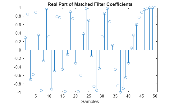
Obtain the matched filter coefficients for the linear FM waveform. The length of the matched filter coefficients is the length of the pulse.

mfcoeffs = getMatchedFilter(waveform);
stem(real(mfcoeffs))
xlabel('Samples')
title('Real Part of Matched Filter Coefficients')

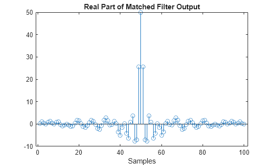
Use the phased.MatchedFilter System object™ to obtain the matched filter output.

mfilter = phased.MatchedFilter('Coefficients',mfcoeffs);
mfoutput = mfilter(wav);
stem(real(mfoutput))
xlabel('Samples')
title('Real Part of Matched Filter Output')

Algorithms

Spectrum weighting produces a matched filter transfer function

$$H\text{'}(F)=w(F)H(F)$$

where w(F) is the window and H(F) is the original transfer function.

For a discussion of matched filter theory, see [1] or [2]. The filtering operation uses the overlap-add method [3].

References

[1] Richards, M. A. Fundamentals of Radar Signal Processing. New York: McGraw-Hill, 2005.

[2] Skolnik, M. Introduction to Radar Systems, 3rd Ed. New York: McGraw-Hill, 2001.

[3] Alan Oppenheim and Ronald Schafer, Discrete-Time Signal Processing, Prentice Hall, 1989.

Extended Capabilities

C/C++ Code Generation

Generate C and C++ code using MATLAB® Coder™.

Usage notes and limitations:

• The CustomSpectrumWindow property is not supported.

• See System Objects in MATLAB Code Generation (MATLAB Coder).

Version History

Introduced in R2011a