Waveform Design for a Dual-Function MIMO RadCom System
This example shows how to design a set of waveforms for a dual-function multiple-input-multiple-output (MIMO) radar-communication (RadCom) system. It then uses the designed waveforms to simulate a RadCom system that can detect targets in range and azimuth, as well as transmit data to multiple downlink users.
Joint Radar-Communication
Radar systems require large bandwidth to achieve high resolution while communication systems require large bandwidth to achieve high data rates. With a growing number of connected devices, the frequency spectrum becomes increasingly congested. To make the frequency spectrum usage more efficient the radar and the communication communities have recently proposed a host of approaches for radar-communication coexistence. These approaches range from non-cooperative spectrum sharing that rely on spectrum sensing and dynamic spectrum access to joint RadCom systems optimized for both functions [1].

This example shows how to design a set of dual-function waveforms for a joint RadCom system. This RadCom system uses a phased array to facilitate MIMO communication. It also takes advantage of waveform diversity to achieve good radar performance. Assume the carrier frequency is 6GHz, the peak transmit power is 0.5 MW, and the same uniform linear array (ULA) is used for transmitting and receiving. Create a ULA with = 16 isotropic antenna elements spaced half of a wavelength apart.
rng('default');                     % Set random number generator for reproducibility

fc = 6e9;                           % Carrier frequency (Hz)
Pt = 0.5e6;                         % Peak transmit power (W)
lambda = freq2wavelen(fc);          % Wavelength (m)

N = 16;                             % Number of array elements
d = 0.5*lambda;                     % Array element spacing (m)

% Use isotropic antenna elements
element = phased.IsotropicAntennaElement('BackBaffled', true);
array = phased.ULA('Element', element, 'NumElements', N, 'ElementSpacing', d, 'ArrayAxis', 'y');
Since the objectives of the radar and the communication components of the RadCom system are fundamentally different, each component imposes different requirements on the transmitted waveforms.
Objective of the Radar Component
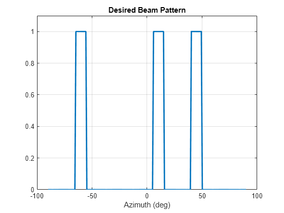
The goal of the Rad component is to form multiple transmit beams in the directions of targets of interest (for example, the tracker subsystem can provide predicted target positions).
Create a desired transmit beam pattern with 10 degree beams pointing at each target.
% Three targets of interest
tgtAz = [-60 10 45];                % Azimuths of the targets of interest
tgtRng = [5.31e3, 6.23e3, 5.7e3];   % Ranges of the targets of interest

ang = linspace(-90, 90, 200);       % Grid of azimuth angles
beamwidth = 10;                     % Desired beamwidth

% Desired beam pattern
idx = false(size(ang));
for i = 1:numel(tgtAz)
    idx = idx | ang >= tgtAz(i)-beamwidth/2 & ang <= tgtAz(i)+beamwidth/2;
end

Bdes = zeros(size(ang));
Bdes(idx) = 1;

figure
plot(ang, Bdes, 'LineWidth', 2)
xlabel('Azimuth (deg)')
title('Desired Beam Pattern')
grid on
ylim([0 1.1])
Objective of the Communication Component
The goal of the Com component is to transmit communication symbols to downlink users. Let there be K=4 single-antenna users and a communication message consisting of M=30 symbols. Create a K-by-M matrix S of QPSK symbols that represents the desired communication message.
K = 4;                              % Number of communication users
M = 30;                             % Number of communication symbols

Q = 4;
data = randi([0 Q-1], K, M);        % Binary data
S = pskmod(data, Q, pi/Q);          % QPSK symbols
Create a K-by-N matrix H that models a scattering channel between N RadCom antenna elements and K downlink users. This matrix is typically assumed to be known to the RadCom system prior to the waveform design.
% User locations are random
txpos = [rand(1, K)*1.5e3; rand(1, K)*2.4e3 - 1.2e3; zeros(1, K)];

% Create a scattering channel matrix assuming 100 independent scatterers
numscat = 100;
rxpos = array.getElementPosition();
H = scatteringchanmtx(rxpos, txpos, numscat).'
H = 4×16 complex

   8.7091 +12.7370i   7.6595 +12.5373i   6.6720 +12.2755i   5.7670 +11.9572i   4.9634 +11.5890i   4.2779 +11.1784i   3.7251 +10.7339i   3.3168 +10.2644i   3.0620 + 9.7795i   2.9665 + 9.2892i   3.0330 + 8.8035i   3.2607 + 8.3323i   3.6456 + 7.8853i   4.1802 + 7.4718i   4.8542 + 7.1005i   5.6539 + 6.7792i
   7.8735 - 1.4713i   7.5420 - 1.0739i   7.1921 - 0.6758i   6.8253 - 0.2874i   6.4428 + 0.0807i   6.0457 + 0.4185i   5.6350 + 0.7169i   5.2113 + 0.9675i   4.7751 + 1.1634i   4.3269 + 1.2988i   3.8668 + 1.3693i   3.3947 + 1.3724i   2.9107 + 1.3070i   2.4146 + 1.1738i   1.9061 + 0.9752i   1.3852 + 0.7152i
   4.5272 -11.8564i   4.4023 -11.2418i   4.2990 -10.5969i   4.2204 - 9.9349i   4.1690 - 9.2692i   4.1469 - 8.6130i   4.1556 - 7.9794i   4.1958 - 7.3807i   4.2677 - 6.8284i   4.3704 - 6.3330i   4.5025 - 5.9036i   4.6617 - 5.5481i   4.8449 - 5.2727i   5.0484 - 5.0820i   5.2675 - 4.9789i   5.4973 - 4.9645i
  -2.6693 - 4.1227i  -2.8238 - 3.8097i  -2.8926 - 3.5504i  -2.8724 - 3.3435i  -2.7609 - 3.1862i  -2.5574 - 3.0744i  -2.2627 - 3.0028i  -1.8792 - 2.9653i  -1.4108 - 2.9546i  -0.8630 - 2.9630i  -0.2427 - 2.9824i   0.4415 - 3.0044i   1.1800 - 3.0207i   1.9620 - 3.0231i   2.7756 - 3.0040i   3.6082 - 2.9564i
Next, the example will show how to create a set of radar waveforms that satisfy the radar objective and form the desired transmit beam pattern. It will then show how to embed the desired communication message into the synthesized waveforms. Finally, the example will model a transmission from the RadCom system. It will plot the resulting range-angle response and compute the symbol error rate to verify that the system is capable of performing both functions.
MIMO Radar Waveform Synthesis
The Rad component of the RadCom system is a MIMO radar. Unlike a traditional phased array radar that transmits a scaled version of the same waveform from each antenna element, a MIMO radar utilizes waveform diversity and transmits different waveforms. These waveforms combine to form the transmit beam pattern. By adjusting the transmitted waveforms, a MIMO radar can dynamically adjust its transmit beam pattern.
Let an -by- matrix represent the transmitted waveforms such that the rows of correspond to the antenna elements and the columns of to subpulses. The resulting transmit beam pattern is [2]
where is the array steering vector, is the azimuth angle, and is the waveform covariance matrix. This relationship shows that design of a transmit beam pattern for a MIMO radar is equivalent to designing the waveform covariance matrix. Therefore, the waveform design process can be broken into two steps. First, you find a covariance matrix that produces the desired beam pattern, and then synthesize the waveforms based on the found covariance matrix. Designing the covariance matrix first is much easier compared to selecting the waveforms directly, since typically , and thus has much fewer unknowns than .
From Beam Pattern to Covariance Matrix
Given a desired beam pattern , a waveform covariance matrix can be found by minimizing the squared error between the desired and the actual beam pattern [2]
s.t.
where is the total transmit power. The first constraint in this optimization problem requires that the diagonal elements of are equal to . This guarantees that each antenna element transmits equal power, and the total transmitted power is equal to . The second constraint restricts to the set of positive semidefinite matrices, which is a necessary requirement for a valid covariance matrix. Use the helperMMSECovariance helper function to solve this optimization problem for the desired beam pattern in Bdes. The solution is the optimal covariance matrix Rmmse that results in a beam pattern closest to the desired beam pattern in the minimum mean squared error (MMSE) sense.
% Normalize the antenna element positions by the wavelength
normalizedPos = rxpos/lambda;

% Solve the optimization problem to find the covariance matrix
Rmmse = helperMMSECovariance(normalizedPos, Bdes, ang);

% helperMMSECovariance returns a covariance matrix with 1s along the
% diagonal such that the total transmit power is equal to N. Renormalize
% the covariance matrix to make the total transmit power equal to Pt.
Rmmse = Rmmse*Pt/N;

% Matrix of steering vectors corresponding to the angles in the grid ang
A = steervec(normalizedPos, [ang; zeros(size(ang))]);

% Compute the resulting beam pattern given the found covariance matrix
Bmmse = abs(diag(A'*Rmmse*A))/(4*pi);
Compare the beam pattern obtained by optimization of the minimum squared error with the desired beam pattern.
figure
hold on
plot(ang, pow2db(Bdes + eps), 'LineWidth', 2)
plot(ang, pow2db(Bmmse/max(Bmmse)), 'LineWidth', 2)

grid on
xlabel('Azimuth (deg)')
ylabel('(dB)')
legend('Desired', 'MMSE Covariance', 'Location', 'southoutside', 'Orientation', 'horizontal')
ylim([-30 1])
title('Transmit Beam Pattern')

The beam pattern obtained from the covariance matrix in Rmmse has three main lobes that match the main lobes of the desired beam pattern and correspond to the directions of the targets of interest. The resulting sidelobe level depends on the available aperture size.
From Covariance Matrix to Waveform
Once the covariance matrix is known, the problem of synthesizing radar waveforms that produce the desired beam pattern reduces to the problem of finding a set of waveforms with a given covariance . But to be useful in practice these waveforms also must meet a number of constraints. For power-efficient transmission both radar and communication systems typically require the waveforms to have a constant modulus. Since, it might be numerically difficult to find a set of constant modulus waveforms with a given covariance matrix, the waveforms can be constrained in terms of the peak-to-average-power ratio (PAR) instead. The PAR for the th transmitted waveform is
where is the average power, , and . Notice that the diagonal elements of the waveform covariance matrix are equal to the average powers of the waveforms . If each antenna element transmits equal power, and the total transmit power is , then . For a set of waveforms, the following low PAR constraint can be set
This constraint requires that the average power of each waveform in the set is equal to the total power divided by the number of antenna elements and that the power for each subpulse does not exceed the average power by more than a factor of . If is set to 1, the low PAR constraint becomes the constant modulus constraint.
In [3] the authors propose a cyclic algorithm (CA) for synthesizing waveforms given a desired covariance matrix such that the PAR constraint is satisfied. The helper function helperCAWaveformSynthesis implements a version of this algorithm described in [4] that also minimizes the autocorrelation sidelobes for each waveform. Set the parameter to 1.1 and use helperCAWaveformSynthesis to find a set of waveforms that have a covariance matrix equal to the optimal covariance matrix in Rmmse. Set the number of subpulses in the generated waveform to be equal to the number of symbols in the desired communication symbol matrix S.
eta = 1.1;                          % Parameter that controls low PAR constraint

% Find a set of waveform with the covariance equal to Rmmse using the
% cyclic algorithm. The length of each waveform is M.
Xca = helperCAWaveformSynthesis(Rmmse, M, eta);

% Covariance matrix of the computed waveforms
Rca = Xca*Xca'/M;

% The resulting beam pattern
Bca = abs(diag(A'*Rca*A))/(4*pi);
Compare the beam pattern formed by the synthesized waveforms Xca with the beam pattern produced by Rmmse and the desired beam pattern Bdes.
figure
hold on
plot(ang, pow2db(Bdes + eps), 'LineWidth', 2)
plot(ang, pow2db(Bmmse/max(Bmmse)), 'LineWidth', 2)
plot(ang, pow2db(Bca/max(Bca)), 'LineWidth', 2)

grid on
xlabel('Azimuth (deg)')
ylabel('(dB)')
legend('Desired', 'MMSE Covariance', 'Radar Waveforms', 'Location', 'southoutside', 'Orientation', 'horizontal')
ylim([-30 1])
title('Transmit Beam Pattern')
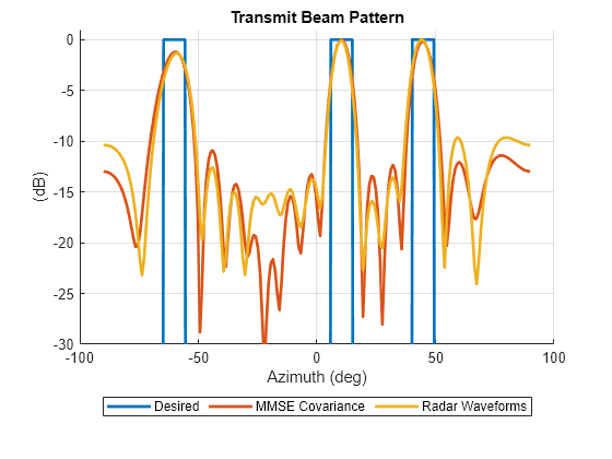
The waveforms synthesized by CA form a beam pattern close to the beam pattern produced by Rmmse. Some distortion is present, but the main lobes are mostly undistorted. Since the diagonal elements of Rmmse were constraint to be equal to , the synthesized waveforms Xca must have average power equal to 0.5e6/16=31250 watt. Verify that the defined low PAR constraint is satisfied for all synthesized waveforms.
% Average power
Pn = diag(Rca);

% Peak-to-average power ratio
PARn = max(abs(Xca).^2, [], 2)./Pn;

array2table([Pn.'; PARn.'], 'VariableNames', compose('%d', 1:N), 'RowNames', {'Average Power', 'Peak-to-Average Power Ratio'})
ans=2×16 table
                                     1        2        3        4        5        6        7        8        9       10       11       12       13       14       15       16
                                   _____    _____    _____    _____    _____    _____    _____    _____    _____    _____    _____    _____    _____    _____    _____    _____

    Average Power                  31250    31250    31250    31250    31250    31250    31250    31250    31250    31250    31250    31250    31250    31250    31250    31250
    Peak-to-Average Power Ratio      1.1      1.1      1.1      1.1      1.1      1.1      1.1      1.1      1.1      1.1      1.1      1.1      1.1      1.1      1.1      1.1
To verify that the generated waveforms have low range sidelobes (an important requirement for a good radar waveform), plot the autocorrelation function for one of the waveforms in Xca. Use the sidelobelevel function to compute the peak-to-sidelobe level (PSL).
% Plot the autocorrelation function for the nth waveform in Xca
n = 1;
[acmag_ca, delay] = ambgfun(Xca(n, :), 1, 1/M, "Cut", "Doppler");
acmag_ca_db = mag2db(acmag_ca);
psl_ca = sidelobelevel(acmag_ca_db);

figure;
ax = gca;
colors = ax.ColorOrder;
plot(delay, acmag_ca_db, 'Color', colors(3, :), 'Linewidth', 2)
yline(psl_ca,'Label',sprintf('Sidelobe Level (%.2f dB)', psl_ca))
xlabel('Lag (subpulses)')
ylabel('(dB)')
title(sprintf('Autocorrelation Function for Waveform #%d', n))
grid on;
ylim([-45 0]);
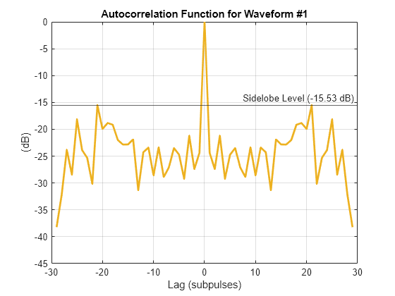
The PSL for the generated waveform is -13.85 dB, which is slightly lower than the PSL of a rectangular LFM pulse.
Radar-Communication Waveform Synthesis
The RadCom system uses the same waveforms for joint radar and communication. If is a known channel matrix and is a matrix containing transmitted waveforms, the signal received by the downlink users is a product . One way to design a set of dual-function waveforms is to embed the communication symbols into the radar waveforms such that the received signal is as close as possible to the set of the desired communication symbols . In other words, such that the difference is minimized. This difference is known as the multi-user interference (MUI).
A set of suitable waveforms is a solution to the following tradeoff objective function with two terms: the first term is the MUI, while the second term represents the mismatch between the desired and the resulting beam pattern
s.t.
here is the initial set of radar waveforms that form the desired beam pattern and is a parameter controlling the tradeoff between the radar and the communication function. Again, the constraint in this optimization problem guarantees that all antenna elements transmit equal power, and the total power is equal to .
If is close to zero, the obtained waveforms will be as close as possible to the initial radar waveforms guaranteeing a good radar performance. However, the MUI in this case can be high resulting in a poor communication performance. When is close to one, the MUI minimization is prioritized resulting in a good communication performance, but possibly poor radar performance. In this case the resulting waveforms might diverge significantly from the initial radar waveforms and therefore the resulting beam pattern might be significantly different from the desired beam pattern.
Authors in [5] use the Riemannian Conjugate Gradient (RCG) method to solve the tradeoff optimization and find a set of dual-function waveforms. Use the helperRadComWaveform helper function that implements the RCG method to embed the 4-by-30 set of QPSK symbols S into the set of synthesized radar waveforms Xca using the generated 4-by-16 channel matrix H.
% Radar-communication tradeoff parameter
rho = 0.4;

% Use RCG to embed the communication symbols in S into the waveforms in Xca
% assuming known channel matrix H.
Xradcom = helperRadComWaveform(H, S, Xca, Pt, rho);

% Compute the corresponding waveform covariance matrix and the transmit beam pattern
Rradcom = Xradcom*Xradcom'/M;
Bradcom = abs(diag(A'*Rradcom*A))/(4*pi);
Compare the beam pattern formed by the obtained waveforms Xradcom against the desired beam pattern Pdes, the beam pattern obtained using the optimal covariance matrix Rmmse, and the beam pattern formed by the radar waveforms Xca generated by CA.
figure;
hold on;
plot(ang, pow2db(Bdes + eps), 'LineWidth', 2);
plot(ang, pow2db(Bmmse/max(Bmmse)), 'LineWidth', 2);
plot(ang, pow2db(Bca/max(Bca)), 'LineWidth', 2);
plot(ang, pow2db(Bradcom/max(Bradcom)), 'LineWidth', 2);

grid on;
xlabel('Azimuth (deg)');
ylabel('(dB)');
legend('Desired', 'MMSE Covariance', 'Radar Waveforms', 'RadCom Waveforms',...
    'Location', 'southoutside', 'Orientation', 'horizontal', 'NumColumns', 2)
ylim([-30 1])
title('Transmit Beam Pattern')
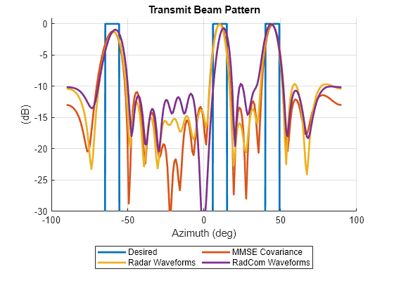
Embedding communication data into the radar waveform causes some transmit beam pattern distortion, however the main lobes are not affected in a significant way. To show the effect of MUI minimization compare the autocorrelation functions of a dual-function waveform in Xradcom and its radar counterpart from Xca. Use the sidelobelevel function to compute the PSL of the dual-function waveform.
[acmag_rc, delay] = ambgfun(Xradcom(n, :), 1, 1/M, "Cut", "Doppler");
acmag_rc_db = mag2db(acmag_rc);
psl_rc = sidelobelevel(acmag_rc_db);

figure
ax = gca;
colors = ax.ColorOrder;

hold on;
plot(delay, acmag_ca_db, 'Color', colors(3, :), 'LineWidth', 2)
plot(delay, acmag_rc_db, 'Color', colors(4, :), 'LineWidth', 2)
yline(psl_rc,'Label',sprintf('Sidelobe Level (%.2f dB)', psl_rc))
xlabel('Lag (subpulses)')
ylabel('(dB)')
title(sprintf('Autocorrelation Function for Waveform #%d', n))
grid on;
ylim([-30 0]);

legend('Radar Waveform', 'RadCom Waveform');
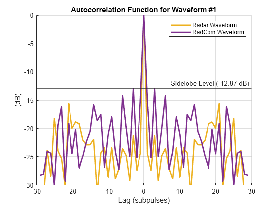
It is evident that after embedding the communication information into the radar waveform the close range sidelobes have increased. However, the PSL has not decreased significantly and is still below -13 dB. The behavior of the sidelobes depends on the value of the parameter . In general, increasing results in increased range sidelobes, since more priority is given to the communication function and less to the radar.
Joint Radar-Communication Simulation
You will use the designed dual-function waveforms to compute a range-angle response and a symbol error rate. Assume that the RadCom system is located at the origin. Let the duration of each subpulse be =0.25s. This means that the bandwidth of the system is =4 MHz. Let the pulse repetition frequency be equal to 15 KHz.
tau = 5e-7;                         % Subpulse duration
B = 1/tau;                          % Bandwidth
prf = 15e3;                         % PRF
fs = B;                             % Sample rate

% The RadCom system is located at the origin and is not moving
radcompos = [0; 0; 0];
radcomvel = [0; 0; 0];
From each antenna element of the transmit array transmit a pulse that consists of the corresponding dual-function waveform.
t = 0:1/fs:(1/prf);

waveform = zeros(numel(t), N);
waveform(1:M, :) = Xradcom' / sqrt(Pt/N);

transmitter = phased.Transmitter('Gain', 0, 'PeakPower', Pt/N, 'InUseOutputPort', true);
txsig = zeros(size(waveform));
for n = 1:N
    txsig(:, n) = transmitter(waveform(:, n));
end
Radiate the transmitted pulses and propagate them towards the targets through a free space channel.
% Positions of the targets of interest in Cartesian coordinates
[x, y, z] = sph2cart(deg2rad(tgtAz), zeros(size(tgtAz)), tgtRng);
tgtpos = [x; y; z];

% Assume the targets are static
tgtvel = zeros(3, numel(tgtAz));

% Calculate the target angles as seen from the transmit array
[tgtRng, tgtang] = rangeangle(tgtpos, radcompos);

radiator = phased.Radiator('Sensor', array, 'OperatingFrequency', fc, 'CombineRadiatedSignals', true);
radtxsig = radiator(txsig, tgtang);

channel = phased.FreeSpace('SampleRate', fs, 'TwoWayPropagation', true, 'OperatingFrequency',fc);
radtxsig = channel(radtxsig, radcompos, tgtpos, radcomvel, tgtvel);
Reflect the transmitted pulses off the targets and receive the reflected echoes by the receive array.
% Target radar cross sections
tgtRCS = [2.7 3.1 4.3];

% Reflect pulse off targets
target = phased.RadarTarget('Model', 'Nonfluctuating', 'MeanRCS', tgtRCS, 'OperatingFrequency', fc);
tgtsig = target(radtxsig);

% Receive target returns at the receive array
collector = phased.Collector('Sensor', array, 'OperatingFrequency', fc);
rxsig = collector(tgtsig, tgtang);

receiver = phased.ReceiverPreamp('Gain', 0, 'NoiseFigure', 2.7, 'SampleRate', fs);
rxsig = receiver(rxsig);
Process the received pulses by computing the range-angle response.
% Compute range-angle response
rngangresp = phased.RangeAngleResponse(...
    'SensorArray',array,'OperatingFrequency',fc,...
    'SampleRate',fs,'PropagationSpeed',collector.PropagationSpeed);

resp = zeros(numel(t), rngangresp.NumAngleSamples, N);

% Apply matched filter N times. One time for each waveform. Then integrate
% the results.
for i = 1:N
    [resp(:, :, i), rng_grid, ang_grid] = rngangresp(rxsig, flipud(Xradcom(i, :).'));
end

% Plot the range angle response
figure
resp_int = sum(abs(resp).^2, 3);
resp_max = max(resp_int, [], 'all');
imagesc(ang_grid, rng_grid, pow2db(resp_int/resp_max))
clim([-20 1])
axis xy
xlabel('Azimuth (deg)')
ylabel('Range (m)')
title('Range-Angle Response')
cbar = colorbar;
cbar.Label.String = '(dB)';

All three targets of interest are visible on the range-angle response. Now, transmit the dual-function waveforms through the MIMO scattering channel H and compute the resulting error rate.
rd = pskdemod(H*Xradcom, Q, pi/Q);
[numErr, errRatio] = symerr(data, rd)
numErr =
27
errRatio =
0.2250
The error rate is close to 4.2%. Note that the resulting performance heavily depends on the tradeoff parameter . To show this for different values of compute the symbol error rate, the PSL of the range response (averaged over N waveforms), and the squared error between the desired beam pattern and the beam pattern formed by the dual-function waveforms.
% Vary the radar-communication tradeoff parameter from 0 to 1
rho = 0.0:0.1:1;

er = zeros(size(rho));
psl_ca = zeros(size(rho));
bpse = zeros(size(rho));

for i = 1:numel(rho)
    Xrc = helperRadComWaveform(H, S, Xca, Pt, rho(i));

    % Transmit through the communication channel and compute the error
    % rate
    rd = pskdemod(H*Xrc, Q, pi/Q);
    [~, er(i)] = symerr(data, rd);

    % Compute the peak to sidelobe level
    psl_ca(i) = helperAveragePSL(Xrc);

    % Compute the beam pattern
    Rrc = Xrc*Xrc'/M;
    Brc = abs(diag(A'*Rrc*A))/(4*pi);

    % Squared error between the desired beam pattern and the beam pattern produced by the RadCom waveforms Xrc
    bpse(i) = trapz(deg2rad(ang), (Bdes.' - Brc/max(Brc)).^2.*cosd(ang).');
end
figure;
tiledlayout(3, 1);

ax = nexttile;
semilogy(rho, er, 'LineWidth', 2);
xlim([0 1]);
ylim([1e-3 1]);
grid on;
title('Symbol Error Rate');

nexttile;
plot(rho, psl_ca, 'LineWidth', 2);
ylabel('(dB)');
grid on;
title({'Peak to Sidelobe Level', '(averaged over 16 waveforms)'});

nexttile;
plot(rho, pow2db(bpse), 'LineWidth', 2);
ylabel('(dB)');
grid on;
title('Squared Error Between the Desired and the RadCom Beam Patterns');

xlabel('\rho');
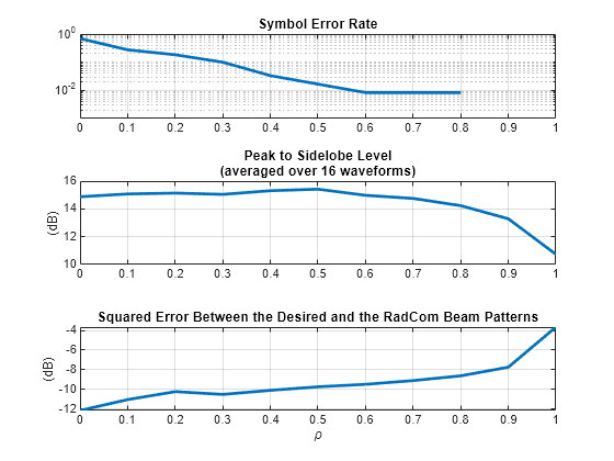
Increasing decreases the symbol error rate. When is equal to 0.8 or larger the symbol error rate becomes zero. This is due to a relatively small number of transmitted symbols used in this simulation. On the other hand, increasing results in the higher sidelobes and a large error between the desired and the resulting transmit beam pattern. By carefully selecting a balance between the radar and the communication performance can be achieved such that the symbol error rate as well as the sidelobes of the range response and the beam pattern distortion are low.
Conclusions
This example shows how to design a set of dual-function waveforms for a joint MIMO RadCom system. The resulting waveforms must form a desired beam pattern to steer transmit beams towards multiple radar targets of interest and transmit a desired symbol matrix to the downlink users over a known MIMO channel. First, the example shows how to synthesize a set of radar waveforms that produce the desired transmit beam pattern. Then, the communication symbols are embedded into the synthesized radar waveforms such that the multi-user interference and the distortions in the transmit beam pattern are minimized. The example then simulates a transmission of the designed waveforms and computes the resulting range-angle response and symbol error rate.
References
Martone, Anthony, and Moeness Amin. "A view on radar and communication systems coexistence and dual functionality in the era of spectrum sensing." Digital Signal Processing 119 (2021): 103135.
Fuhrmann, Daniel R., and Geoffrey San Antonio. "Transmit beamforming for MIMO radar systems using signal cross-correlation." IEEE Transactions on Aerospace and Electronic Systems 44, no. 1 (2008): 171-186.
Stoica, Petre, Jian Li, and Xumin Zhu. "Waveform synthesis for diversity-based transmit beampattern design." IEEE Transactions on Signal Processing 56, no. 6 (2008): 2593-2598.
He, Hao, Jian Li, and Petre Stoica. Waveform design for active sensing systems: a computational approach. Cambridge University Press, 2012.
Liu, Fan, Longfei Zhou, Christos Masouros, Ang Li, Wu Luo, and Athina Petropulu. "Toward dual-functional radar-communication systems: Optimal waveform design." IEEE Transactions on Signal Processing 66, no. 16 (2018): 4264-4279.
Supporting Functions
type 'helperMMSECovariance.m'function R = helperMMSECovariance(elPos, Pdesired, ang)
% This function computes a waveform covariance matrix that generates a
% desired transmit beam pattern. The computation is based on the squared
% error optimization described in
%
% Fuhrmann, Daniel R., and Geoffrey San Antonio. "Transmit beamforming for
% MIMO radar systems using signal cross-correlation." IEEE Transactions on
% Aerospace and Electronic Systems 44, no. 1 (2008): 171-186.
%
% elPos is a 3-by-N matrix of array element positions normalized by the
% wavelength. Pdesired is the desired beam pattern evaluated at the angles
% specified in ang.
N = size(elPos, 2);
% Initial covariance is random. x_ is a vector of all elements that are
% in the upper triangular part of the matrix above the main diagonal.
x_ = initialCovariance(N);
% Normalized the desired beam pattern such that the total transmit power is
% equal to the number of array elements N.
Pdesired = N * Pdesired / (2*pi*trapz(deg2rad(ang), Pdesired.*cosd(ang)));
Pdesired = Pdesired * 4 * pi;
% Matrix of steering vectors corresponding to angles in ang
A = steervec(elPos, [ang; zeros(size(ang))]);
% Parameters of the barrier method
mu = 4;
% The barrier term is weighted by 1/t. At each iteration t is multiplied
% by mu to decrease the contribution of the barrier function.
t = 0.02;
epsilon = 1e-1;
stopCriteriaMet = false;
J_ = squaredErrorObjective(x_, t, A, Pdesired, ang);
while ~stopCriteriaMet
% Run Newton optimization using x_ as a starting point
x = newtonOptimization(x_, t, A, Pdesired, ang);
J = squaredErrorObjective(x, t, A, Pdesired, ang);
if abs(J) < abs(J_)
stopCriteriaMet = abs(J - J_) < epsilon;
x_ = x;
J_ = J;
else
% Increased t by too much, step back a little.
t = t / mu;
mu = max(mu * 0.8, 1.01);
end
t = t * mu;
end
R = constrainedCovariance(x, N);
end
function x = newtonOptimization(x_, t, A, Pdesired, ang)
epsilon = 1e-3;
% Parameters for Armijo rule
s = 2;
beta = 0.5;
sigma = 0.1;
stopCriteriaMet = false;
J_ = squaredErrorObjective(x_, t, A, Pdesired, ang);
while ~stopCriteriaMet
[g, H] = gradientAndHessian(x_, t, A, Pdesired, ang);
% Descent direction
d = -(H\g);
% Compute step size and the new value x using the Armijo rule
m = 0;
gamma = g'*d;
while true
mu = (beta^m)*s;
x = x_ + mu*d;
J = squaredErrorObjective(x, t, A, Pdesired, ang);
if abs(J_) - abs(J) >= (-sigma*mu*gamma)
x_ = x;
stopCriteriaMet = abs(J - J_) < epsilon;
J_ = J;
break;
end
m = m + 1;
end
end
end
function [G, H] = gradientAndHessian(x, t, A, Pdesired, ang)
N = size(A, 1);
M = N*(N-1);
F = constrainedCovariance(x, N);
numAng = numel(ang);
FinvFi = zeros(N, N, M);
Alpha = zeros(M, numAng);
idxs = find(triu(ones(N, N), 1));
[r, c] = ind2sub([N N], idxs);
for i = 1:M/2
[Fi_re, Fi_im] = basisMatrix(N, r(i), c(i));
% Matrix inverses used in Eq. (26) and (27)
FinvFi(:, :, i) = F\Fi_re;
FinvFi(:, :, i + M/2) = F\Fi_im;
% Eq. (29)
Alpha(i, :) = 2*real(conj(A(r(i), :)) .* A(c(i), :));
Alpha(i + M/2, :) = -2*imag(conj(A(r(i), :)) .* A(c(i), :));
end
G = zeros(M, 1);
H = zeros(M, M);
D = (real(diag(A'*F*A).') - Pdesired) .* cosd(ang);
ang_rad = deg2rad(ang);
for i = 1:M
% Eq. (33a)
G(i) = -trace(squeeze(FinvFi(:, :, i))) * (1/t) + 2*trapz(ang_rad, Alpha(i, :) .* D);
for j = i:M
% Eq. (33b)
H(i, j) = trace(squeeze(FinvFi(:, :, i))*squeeze(FinvFi(:, :, j))) * (1/t) ...
+ 2*trapz(ang_rad, Alpha(i, :).*Alpha(j, :).*cosd(ang));
end
end
H = H + triu(H, 1)';
end
function [Fi_re, Fi_im] = basisMatrix(N, i, j)
Fi_re = zeros(N, N);
Fi_re(i, j) = 1;
Fi_re(j, i) = 1;
Fi_im = zeros(N, N);
Fi_im(i, j) = 1i;
Fi_im(j, i) = -1i;
end
function J = squaredErrorObjective(x, t, A, Pdesired, ang)
% Squared error between the desired beam pattern in Pdesired and the
% beam pattern formed by a covariance matrix defined by the vector x
% containing the above diagonal elements
N = size(A, 1);
% Beam patter defined by x
F = constrainedCovariance(x, N);
P_ = real(diag(A'*F*A).');
% Squared error weighted by angle
E = abs(Pdesired - P_).^2 .* cosd(ang);
% Total error over all angles
J = trapz(deg2rad(ang), E);
% Barrier function
d = eig(F);
if all(d >= 0)
phi = -log(prod(d));
else
phi = Inf;
end
J = J + (1/t)*phi;
end
function F = constrainedCovariance(x, N)
% Reconstruct the covariance matrix from a vector x of above diagonal
% values. The diagonal elements are all equal to 1.
Re = zeros(N, N);
Im = zeros(N, N);
M = numel(x);
idxs = triu(ones(N, N), 1) == 1;
Re(idxs) = x(1:M/2);
Im(idxs) = x(M/2+1:end);
F = eye(N, N);
F = F + Re + Re.' + 1i*Im - 1i*Im.';
end
function x = initialCovariance(N)
% Create a random covariance matrix
X = randn(N, 10*N) + 1i*randn(N, 10*N);
L = sum(conj(X) .* X, 2);
X = X./sqrt(L);
R = X*X';
M = N*(N-1);
x = zeros(M, 1);
% Select the elements that are above the main diagonal
idxs = triu(ones(N, N), 1) == 1;
x(1:M/2) = real(R(idxs));
x(M/2+1:end) = imag(R(idxs));
end
type 'helperCAWaveformSynthesis.m'function X = helperCAWaveformSynthesis(R, M, rho)
% This function generates a set of waveforms that form the desired
% covariance matrix R. M is the number of waveform samples and rho is a
% parameter controlling the resulting peak-to-average power ratio (PAR).
% This algorithm is described in the chapter 14 of
%
% He, Hao, Jian Li, and Petre Stoica. Waveform design for active sensing
% systems: a computational approach. Cambridge University Press, 2012.
%
% and in
%
% Stoica, Petre, Jian Li, and Xumin Zhu. "Waveform synthesis for
% diversity-based transmit beampattern design." IEEE Transactions on Signal
% Processing 56, no. 6 (2008): 2593-2598.
N = size(R, 1);
epsilon = 0.1;
% P can control the autocorrelation level for each waveform. If P = M the
% optimization is trying to minimize sidelobes for across all M-1 lags.
P = M;
% Arbitrary semi-unitary matrix
U = (randn(P + M - 1, N*P) + 1i*randn(P + M - 1, N*P))/sqrt(2);
% Expended covariance is used to minimize the autocorrelation sidelobes. See
% eq. (14.10) and (14.11)
Rexp = kron(R, eye(P));
% Square root of the expended covariance
[L, D] = ldl(Rexp);
Rexp_sr = sqrt(D)*L';
% Cyclic algorithm
numIter = 0;
maxNumIter = 1000;
while true
% Z has waveforms that form R but do not satisfy the PAR constraint
% Eq. (14.6)
Z = sqrt(M) * U * Rexp_sr;
X = zeros(M, N);
Xexp = zeros(P + M - 1, N*P);
% Go through each waveform
for n = 1:N
% Retrieve the nth waveform from the expended matrix Z
zn = getzn(Z, M, P, n);
gamma = R(n, n);
% Enforces PAR constraint using nearest vector algorithm
xn = nearestVector(zn, gamma, rho);
X(:, n) = xn;
% Compute new expended waveform matrix
for p = 1:P
Xexp(p:p+M-1, (n-1)*P + p) = xn;
end
end
% Recompute U. Eq. (5) and (11) in the paper
[Ubar, ~, Utilde] = svd(sqrt(M)*Rexp_sr*Xexp', 'econ');
U_ = Utilde * Ubar';
numIter = numIter + 1;
if norm(U-U_) < epsilon || numIter > maxNumIter
break;
else
U = U_;
end
end
X = X';
end
function zn = getzn(Z, M, P, n)
zn = zeros(M, P);
for i = 1:P
zn(:, i) = Z(i:i+M-1, (n-1)*P + i);
end
zn = mean(zn, 2);
end
% Nearest vector algorithm, pages 70-71
function z = nearestVector(z, gamma, rho)
M = numel(z);
S = z'*z;
z = sqrt(M*gamma/S)*z;
beta = gamma * rho;
if all(abs(z).^2 <= beta)
return;
else
ind = true(M, 1);
for i = 1:M
[~, j] = max(abs(z).^2);
z(j) = sqrt(beta)*exp(1i*angle(z(j)));
ind(j) = false;
S = z(ind)'*z(ind);
z(ind) = sqrt((M-i*rho)*gamma/S)*z(ind);
if all(abs(z(ind)).^2 <= (beta+eps))
return;
end
end
end
end
type 'helperRadComWaveform.m'function X = helperRadComWaveform(H, S, X0, Pt, rho)
% This function implements Riemannian Conjugate Gradient (RCG) algorithm
% described in
%
% Liu, Fan, Longfei Zhou, Christos Masouros, Ang Li, Wu Luo, and Athina
% Petropulu. "Toward dual-functional radar-communication systems: Optimal
% waveform design." IEEE Transactions on Signal Processing 66, no. 16
% (2018): 4264-4279.
%
% H is a K-by-N channel matrix where K is the number of down-link users
% and N is the number of antennas at the RadCom base station. S is a K-by-L
% symbol matrix, where L is the number of symbols. X0 is a N-by-L matrix of
% waveforms that generate the desired radar beam pattern. Pt is total
% transmit power, and rho is a trade-off parameter to balance the radar and
% communication performance.
delta = 0.5e-6;
maxNumIterations = 600;
[N, M] = size(X0);
S = S * sqrt(Pt/size(S, 1));
A = [sqrt(rho)*H; sqrt(1-rho)*eye(N)];
B = [sqrt(rho)*S; sqrt(1-rho)*X0];
X = (randn(N, M) + 1i*randn(N, M))/sqrt(2);
X = Rx(X, 0, Pt);
% Euclidean gradient
dF = 2 * A' * (A * X - B);
% Projection of the gradient onto the tangent space at X
gradF = Px(X, dF, Pt);
% Descent direction
G = -gradF;
% Armijo rule parameters
s = 1;
beta = 0.5;
sigma = 0.01;
k = 1;
while true
fx = norm(A*X-B, 'fro').^2;
% Iterate until the maximum number of iterations is reached or the norm
% of the gradient is less than delta
if k > maxNumIterations || norm(gradF, 'fro') < delta
break
end
% If the inner product of the gradient and the descent direction is
% positive reset the descent direction and make it equal to the
% negative gradient
gamma = real(trace(gradF*G'));
if gamma > 0
G = -gradF;
gamma = real(trace(gradF*G'));
end
% Step size and new X computation using Armijo rule
m = 0;
mu = 1;
while (-sigma*mu*gamma) > 0
mu = (beta^m)*s;
X_ = Rx(X, mu*G, Pt);
fx_ = norm(A*X_ - B, 'fro').^2;
if (fx(1) - fx_(1)) >= (-sigma*mu*gamma)
X = X_;
break;
end
m = m + 1;
end
% Previous projected gradient
gradF_ = gradF;
% Previous descent direction
G_ = G;
% Euclidean gradient at X
dF = 2 * A' * (A * X - B);
% Projection of the gradient onto the tangent space at X
gradF = Px(X, dF, Pt);
% Polak-Ribiere combination coefficient
tau = real(trace(gradF'* (gradF - Px(X, gradF_, Pt)))) / real(trace(gradF_'*gradF_));
% New descent direction is a combination of the current negative
% gradient and the previous gradient translated into the current
% tangent space
G = -gradF + tau * Px(X, G_, Pt);
k = k + 1;
end
end
% Tangent space projector
function PxZ = Px(X, Z, Pt)
[N, M] = size(X);
d = diag(Z*X');
PxZ = Z - diag(d)*X*(N/(M*Pt));
end
% Retractor mapping
function RxZ = Rx(X, Z, Pt)
[N, M] = size(X);
Y = X + Z;
d = diag(Y*Y').^(-1/2);
RxZ = sqrt(M * Pt / N)*diag(d) * Y;
end
type 'helperAveragePSL.m'function avpsl = helperAveragePSL(X)
[n, m] = size(X);
psl = zeros(n, 1);
for i = 1:n
acmag = ambgfun(X(i, :), 1, 1/m, "Cut", "Doppler");
psl(i) = acmag(m)/max([acmag(1:m-1) acmag(m+1:end)]);
end
avpsl = mag2db(mean(psl));
end