bistaticConstantSNR

Create bistatic constant SNR contours or surfaces

Since R2024b

Syntax

bistaticConstantSNR(txpos,rxpos,K)

bistaticConstantSNR(txpos,rxpos,K,Name=Value)

[M,SNRcusp] = bistaticConstantSNR(txpos,rxpos,K,Name=Value)

Description

Use bistaticConstantSNR to create, plot, and optionally output bistatic constant SNR (Signal to Noise Ratio) contours or surfaces, also known as ovals of Cassini or Cassini surfaces. Unlike for monostatic radars, bistatic radar systems have separate transmitter and receiver elements that are not co-located. The bistaticConstantSNR function assumes the bistatic transmitter and receiver are synchronized.

bistaticConstantSNR(txpos,rxpos,K) creates and plots bistatic constant SNR contours or surfaces for specified transmitter position (txpos), receiver position (rxpos), and bistatic radar constant (K).

bistaticConstantSNR(txpos,rxpos,K,Name=Value) creates and plots bistatic constant SNR contours or surfaces, with additional options specified using one or more name-value arguments.

[M,SNRcusp] = bistaticConstantSNR(txpos,rxpos,K,Name=Value) returns M, a structure that contains bistatic constant SNR contours or surfaces, and SNRcusp, the scalar SNR value at the cusp. This syntax does not produce a plot.

Examples

Plot Constant SNR Contours

This example shows how to plot constant SNR contours (ovals of Cassini) for a bistatic radar and calculate the bistatic radar constant, K.

Calculate Bistatic Radar Constant (K) and Plot Constant SNR Contours

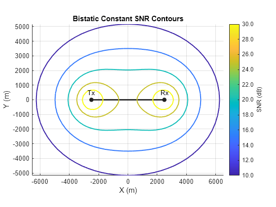
Plot ovals of Cassini for a bistatic radar operating at a frequency of 5.6 GHz and a peak power of 1.5 MW. The transmitter and receiver are 5 km apart. Assume a bistatic target radar cross section (RCS) of 0.1 ${\mathrm{m}}^2$ and a rectangular waveform with a pulse width of 0.2 microseconds. The transmitter gain is 20 dB and the receiver gain is 10 dB. Assume no system loss.

% Inputs
freq   = 5.6e9;              % Radar operating frequency (Hz)
lambda = freq2wavelen(freq); % Wavelength (m)
Pt     = 1.5e6;              % Peak power (W)
tau    = 0.2e-6;             % Pulse width (s)
sigma  = 0.1;                % Bistatic radar cross section (m^2)
Gtx    = 20;                 % Transmitter gain (dB)
Grx    = 10;                 % Receiver gain (dB)
txpos  = [-2.5e3 0];         % Transmitter position (m)
rxpos  = [2.5e3 0];          % Receiver position (m)

% Calculate bistatic radar constant K (dB)
K = radareqsnr(lambda,1,Pt,tau,rcs=sigma,gain=[Gtx Grx]);

% Plot bistatic constant SNR contours
bistaticConstantSNR(txpos,rxpos,K)

Plot Constant SNR Contours for Specified SNR Values

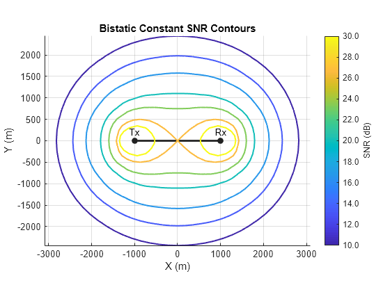
This example shows how to plot constant SNR contours (ovals of Cassini) for a bistatic radar at specified SNR values. Include the cusp that denotes the transmitter-centered and receiver-centered operational regions.

Plot Constant SNR Contours

Plot ovals of Cassini for a bistatic radar that has a bistatic radar constant, K, given by $\mathit{K}=30*{\mathit{L}}^4,$where L is the distance between the transmitter and receiver. Plot contours at SNRs of [10 13 16 20 23 30] and include the cusp.

% Inputs
txpos = [-1e3 0];             % Transmitter position (m)
rxpos = [1e3 0];              % Receiver position (m)
L     = norm(txpos - rxpos);  % Baseline distance (m)
K     = pow2db(30*L^4);       % Bistatic radar constant K (dB)
SNRs  = [10 13 16 20 23 30];  % SNRs (dB)

% Plot bistatic constant SNR contours
bistaticConstantSNR(txpos,rxpos,K,SNR=SNRs,IncludeCusp=true)

Plot Constant SNR Surfaces for Specified Azimuth and Elevation Angles

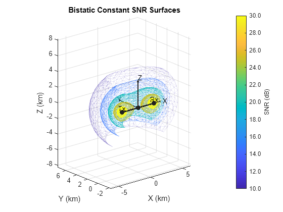
This example shows how to plot constant SNR surfaces (Cassini surfaces) at specified azimuth and elevation angles for a bistatic radar.

Plot Constant SNR Surfaces

Plot Cassini surfaces for a bistatic radar operating at a frequency of 5.6 GHz and a peak power of 1.5 MW. Limit the plot to cover 0 to 180 degrees in azimuth and -45 to 45 degrees in elevation and plot in km. The transmitter and receiver are 5 km apart. Assume a bistatic target RCS of 0.1 ${\mathrm{m}}^2$ and a rectangular waveform with a pulse width of 0.2 microseconds. The transmitter gain is 20 dB and the receiver gain is 10 dB. Assume no system loss.

% Inputs
freq   = 5.6e9;              % Radar operating frequency (Hz)
lambda = freq2wavelen(freq); % Wavelength (m)
Pt     = 1.5e6;              % Peak power (W)
tau    = 0.2e-6;             % Pulse width (s)
sigma  = 0.1;                % Bistatic radar cross section (m^2)
Gtx    = 20;                 % Transmitter gain (dB)
Grx    = 10;                 % Receiver gain (dB)
txpos  = [-2.5e3 0 0];         % Transmitter position (m)
rxpos  = [2.5e3 0 0];          % Receiver position (m)

% Calculate bistatic radar constant K (dB)
K = radareqsnr(lambda,1,Pt,tau,rcs=sigma,gain=[Gtx Grx]);

% Plot bistatic constant SNR surfaces
bistaticConstantSNR(txpos,rxpos,K, ...
   PlotUnits="km",AzimuthLimits=[0 180],ElevationLimits=[-45 45], ...
   ShowLocalCoordinates=true)
view([-40 20])

Output Constant SNR Contour Data and Plot

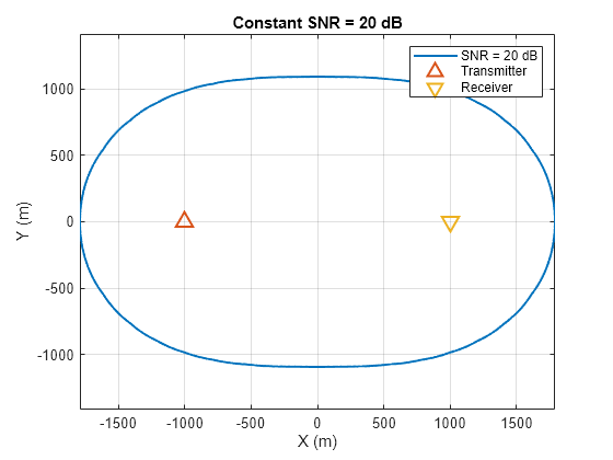
This example shows how to output and manually plot constant SNR contour data for a bistatic radar at a specified SNR value.

Calculate Constant SNR Contour

Calculate the oval of Cassini at an SNR of 20 dB for a bistatic radar that has a bistatic radar constant, K, given by $\mathit{K}=30*{\mathit{L}}^4,$where L is the distance between the transmitter and receiver. Manually plot the results.

% Inputs
txpos = [-1e3 0];             % Transmitter position (m)
rxpos = [1e3 0];              % Receiver position (m)
L     = norm(txpos - rxpos);  % Baseline distance (m)
K     = pow2db(30*L^4);       % Bistatic radar constant K (dB)

% Calculate bistatic constant SNR contour
M = bistaticConstantSNR(txpos,rxpos,K,SNR=20,NumSamples=1e3)

M = struct with fields:
      X: [-1.7892e+03 -1.7892e+03 -1.7890e+03 -1.7886e+03 -1.7882e+03 -1.7876e+03 -1.7869e+03 -1.7861e+03 -1.7852e+03 -1.7841e+03 -1.7829e+03 -1.7816e+03 -1.7801e+03 -1.7785e+03 -1.7768e+03 -1.7749e+03 -1.7730e+03 -1.7709e+03 … ] (1×1028 double)
      Y: [-2.1912e-13 -11.2530 -22.5045 -33.7530 -44.9970 -56.2350 -67.4655 -78.6870 -89.8980 -101.0970 -112.2823 -123.4525 -134.6060 -145.7412 -156.8565 -167.9503 -179.0210 -190.0669 -201.0865 -212.0779 -223.0396 -233.9698 -244.8667 … ] (1×1028 double)
    SNR: 20

% Plot
figure
plot(M.X,M.Y,'LineWidth',1.5)
hold on 
plot(txpos(1),txpos(2),'^','LineWidth',1.5,'MarkerSize',10)
plot(rxpos(1),rxpos(2),'v','LineWidth',1.5,'MarkerSize',10)
grid on
axis equal
xlabel('X (m)')
ylabel('Y (m)')
legend('SNR = 20 dB','Transmitter','Receiver')
title('Constant SNR = 20 dB')

Input Arguments

txpos — Transmitter position (m)

2-element row vector | 3-element row vector

Transmitter position specified as a 2-element or 3-element row vector in global Cartesian coordinates, in units of meters. When txpos is a 2-element row vector, this function plots constant SNR contours. When txpos is a 3-element row vector, this function plots constant SNR surfaces. The length of txpos matches the length of rxpos.

Data Types: double

rxpos — Receiver position (m)

2-element row vector | 3-element row vector

Receiver position specified as a 2-element or 3-element row vector in global Cartesian coordinates, in units of meters. When rxpos is a 2-element row vector, this function plots constant SNR contours. When rxpos is a 3-element row vector, this function plots constant SNR surfaces. The length of rxpos matches the length of txpos.

Data Types: double

K — Bistatic radar constant (dB)

scalar

Scalar bistatic radar constant in dB. See Bistatic Radar Constant (K) for more information.

Data Types: double

Name-Value Arguments

Example: bistaticConstantSNR(txpos,rxpos,K,SNR=20,NumSamples=1e3,NumTrials=100,IncludeCusp=true)

Specify optional pairs of arguments as Name1=Value1,...,NameN=ValueN, where Name is the argument name and Value is the corresponding value. Name-value arguments must appear after other arguments, but the order of the pairs does not matter.

SNR — Signal-to-Noise Ratios for constant SNR contours or surfaces (dB)

[10:5:30] (default) | row vector

Signal-to-Noise Ratios at which to calculate constant SNR contours or surfaces, specified as a row vector in dB. Default is [10:5:30].

Data Types: double

RangeLimits — Range for constant SNR contours or surfaces (m)

[1 100e3] (default) | 2-element positive row vector

Minimum and maximum ranges at which to calculate constant SNR contours or surfaces, specified as [MinRange MaxRange] in meters, where MinRange is the minimum range and MaxRange is the maximum range. The coordinate system is a local coordinate system in which the origin is defined as the midpoint of the bistatic baseline. Default is [1 100e3].

Data Types: double

AzimuthLimits — Azimuth range for constant SNR contours or surfaces (deg)

[-180 180] (default) | 2-element row vector

Minimum and maximum azimuth angles at which to calculate constant SNR contours or surfaces, specified as [MinAzimuth MaxAzimuth], where MinAzimuth is the minimum azimuth and MaxAzimuth is the maximum azimuth. Units are in degrees. Azimuth is the counterclockwise angle measured from the positive x-axis. The positive x-axis is the unit vector pointing from txpos to rxpos. The coordinate system is a local coordinate system in which the origin is defined as the midpoint of the bistatic baseline. Default is [-180 180].

Data Types: double

ElevationLimits — Elevation range for constant SNR contours or surfaces (deg)

[-90 90] (default) | 2-element row vector

Minimum and maximum elevation angles at which to calculate constant SNR surfaces, specified as [MinElevation MaxElevation], where MinElevation is the minimum elevation and MaxElevation is the maximum elevation. Units are in degrees. This property only applies to constant SNR surfaces and is therefore only available when txpos is a 3-element row vector. Elevation is the angle measured from the x-y plane to the positive x-axis. The positive x-axis is the unit vector pointing from txpos to rxpos. The coordinate system is a local coordinate system in which the origin is defined as the midpoint of the bistatic baseline. Default is [-90 90].

Data Types: double

NumSamples — Number of samples

[501 73 37] (default) | 3-element row vector | 2-element row vector | scalar

Number of samples for range, azimuth, and elevation dimensions for the extents defined by the RangeLimits, AzimuthLimits, and ElevationLimits arguments, specified as a scalar or vector.

• Scalar — When NumSamples is specified as a scalar, the same scalar value is applied to all dimensions.

• 2-element row vector — When NumSamples is specified as a 2-element row vector, it has the form [NumSamplesRange NumSamplesAzimuth], where NumSamplesRange is the number of samples in range and NumSamplesAzimuth is the number of samples in azimuth.

• 3-element row vector — When NumSamples is specified as a 3-element row vector, it has the form [NumSamplesRange NumSamplesAzimuth NumSamplesElevation], where NumSamplesRange is the number of samples in range, NumSamplesAzimuth is the number of samples in azimuth, and NumSamplesElevation is the number of samples in the elevation dimension.

The elevation dimension is not relevant to SNR contours. If txpos is a 2-element row vector and NumSamples is specified as a 3-element row vector, the third element of NumSamples is ignored. A 3-element specification for NumSamples is appropriate when txpos is a 3-element row vector for SNR surfaces. Increasing the sampling number, especially in the range dimension, improves accuracy but may decrease performance. The default value is [501 73 37], which results in a resolution of 200 meters in range and 5 degrees in azimuth and elevation for the default range, azimuth, and elevation limits.

Data Types: double

IncludeCusp — Enable cusp inclusion

false (default) | true

Enable the point on the baseline where the ovals or surfaces break into two parts, the cusp, to be included in the plot of the constant SNR contours or surfaces. The cusp occurs at the center of a lemniscate that denotes two distinct operational regions, transmitter-centered and receiver-centered. Set IncludeCusp to true to plot the cusp. Otherwise, the cusp is not considered. The default is false.

Data Types: logical

PlotUnits — Units for the plot

"m" (default) | "km" | "mi" | "nmi" | "ft" | "kft"

Specify units for the plot as one of meter ("m"), kilometer ("km"), mile ("mi"), nautical mile ("nmi"), feet ("ft"), or kilo-feet ("kft"). The default value is "m".

Data Types: string

ShowLocalCoordinates — Enable local coordinate plot axes

false (default) | true

Enable local coordinate axes on the plot. Set ShowLocalCoordinates to true to plot the local coordinate axes. Otherwise, the local coordinate axes are not plotted. The default is false.

Data Types: logical

Parent — Handle to axes in figure

current axes (default) | Axes object

Handle to the plot axes, specified as an Axes object. Use the gca function to get and set properties of the current axes.

Output Arguments

M — Bistatic constant SNR contours or surfaces

structure array

Returns a 1-by-L structure array with three fields that contain coordinate or SNR values that describe each bistatic constant SNR contour or surface, where L is the number of contours or surfaces.

• txpos is a 2-element row vector — For contours, the three fields in M are named X, Y, and SNR. X is a row vector of x-coordinate values (meters), Y is a row vector of y-coordinate values (meters), and SNR is a scalar constant SNR value (dB), for each contour.

• txpos is a 3-element row vector — For surfaces, the three fields in M are named Faces, Vertices, and SNR. Faces is a 3-column matrix where each row corresponds to the face of a polygon, Vertices is a 3-column matrix where each row contains x-, y-, and z-coordinate values (meters) for a vertex, and SNR is a scalar constant SNR value (dB), for each isosurface.

If IncludeCusp is set to true, the output M will include all the user-specified SNRs, as well as the cusp SNR. The coordinate system is a local coordinate system in which the origin is defined as the midpoint of the bistatic baseline. You can use the patch function to plot Faces and Vertices data.

SNRcusp — Cusp (dB)

scalar

Returns the SNR value at the cusp. The cusp is the point on the baseline at which the ovals or surfaces break into two parts, and two distinct operational regions, transmitter-centered and receiver-centered, emerge.

More About

Bistatic Radar Constant (K)

The bistatic radar constant, K, incorporates parameters related to the radar and target and is used to determine the power, or signal, received by the bistatic radar. K is typically defined as

$$K=\frac{P_t{G}_t{G}_r{\lambda }^2\sigma F_t^2{F}_r^2}{{(4\pi )}^{3}k{T}_s{B}_n{L}_t{L}_r},$$

where the terms in the equation are:

• P_t — Transmitter power in watts

• G_t — Transmitter antenna gain

• G_r — Receiver antenna gain

• λ — Radar wavelength in meters

• σ — Target's nonfluctuating Radar Cross Section (RCS) in square meters

• F_t — Propagation factor for the path from the transmitter to the target

• F_r — Propagation factor for the path from the receiver to the target

• k — Boltzmann's constant in joules per kelvin

• T_s — Receiver system noise temperature in kelvin

• B_n — Receiver noise bandwidth in hertz

• L_t — Transmitter loss factor

• L_r — Receiver loss factor

Terms expressed in decibels, such as the loss and gain factors, enter the equation in the form 10^x/10 where x denotes the variable. For example, the default loss factor of 0 dB results in a loss term of 10^0/10=1.

Bistatic Geometry

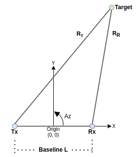
The image below shows the bistatic geometry for the 2-D case. The transmitter and receiver sites reside along the x-axis. In the bistaticConstantSNR function, the positive x-axis is the unit vector pointing from txpos to rxpos. The baseline L, or direct path, is defined as the line between the transmitter Tx and receiver Rx. The line from the transmitter to the target is the range R_T and the range from the receiver to the target is the range R_R. The azimuth is the counterclockwise angle in the x-y plane measured from the positive x-axis, in units of degrees. As shown, the origin for the local coordinate system is the center point of the bistatic baseline L.

An oval of Cassini is the locus of the vertex of a triangle when the product of the sides adjacent to the vertex is constant and the length of the opposite side is fixed [1]. For the bistatic case, the vertex is the target. The sides adjacent to the vertex are R_T and R_R. The baseline L is the fixed, opposite side. The bistatic ovals of Cassini are contours of constant signal-to-noise-ratio (SNR) on any bistatic plane.

SNR = K / (R_T²R_R²),

where K is the bistatic radar constant.

References

[1] Willis, Nicholas J. Bistatic Radar. Raleigh, NC: SciTech Publishing, Inc., 2005.

Version History

Introduced in R2024b