Plan and Execute Task- and Joint-Space Trajectories Using Kinova Gen3 Manipulator
This example shows how to generate and simulate interpolated joint trajectories to move from an initial to a desired end-effector pose. The timing of the trajectories is based on an approximate desired end of arm tool (EOAT) speed.
Load the Kinova® Gen3 rigid body tree (RBT) robot model.
robot = loadrobot('kinovaGen3','DataFormat','row','Gravity',[0 0 -9.81]);
Set current robot joint configuration.
currentRobotJConfig = homeConfiguration(robot);
Get number of joints and the end-effector RBT frame.
numJoints = numel(currentRobotJConfig);
endEffector = "EndEffector_Link";
Specify the trajectory time step and approximate desired tool speed.
timeStep = 0.1; % seconds
toolSpeed = 0.1; % m/s
Set the initial and final end-effector pose.
jointInit = currentRobotJConfig;
taskInit = getTransform(robot,jointInit,endEffector);

taskFinal = trvec2tform([0.4,0,0.6])*axang2tform([0 1 0 pi]);
Generate Task-Space Trajectory
Compute task-space trajectory waypoints via interpolation.
First, compute tool traveling distance.
distance = norm(tform2trvec(taskInit)-tform2trvec(taskFinal));
Next, define trajectory times based on traveling distance and desired tool speed.
initTime = 0;
finalTime = (distance/toolSpeed) - initTime;
trajTimes = initTime:timeStep:finalTime;
timeInterval = [trajTimes(1); trajTimes(end)];
Interpolate between taskInit and taskFinal to compute intermediate task-space waypoints.
[taskWaypoints,taskVelocities] = transformtraj(taskInit,taskFinal,timeInterval,trajTimes);
Control Task-Space Motion
Create a task space motion model for PD control on the joints. The taskSpaceMotionModel object models the motion of a rigid body tree model under task-space proportional-derivative control.
tsMotionModel = taskSpaceMotionModel('RigidBodyTree',robot,'EndEffectorName','EndEffector_Link');
Set the proportional and derivative gains on orientation to zero, so that controlled behavior just follows the reference positions:
tsMotionModel.Kp(1:3,1:3) = 0;
tsMotionModel.Kd(1:3,1:3) = 0;
Define the initial states (joint positions and velocities).
q0 = currentRobotJConfig;
qd0 = zeros(size(q0));
Use ode15s to simulate the robot motion. For this problem, the closed-loop system is stiff, meaning that there is a difference in scaling somewhere in the problem. As a result, the integrator is sometimes forced to take exceedingly small steps, and a non-stiff ODE solver such as ode45 will take much longer to solve the same problem. For more information, refer to Choose an ODE Solver and Solve Stiff ODEs in the documentation.
Since the reference state changes at each instant, a wrapper function is required to update the interpolated trajectory input to the state derivative at each instant. Therefore, an example helper function is passed as the function handle to the ODE solver. The resultant manipulator states are output in stateTask.
[tTask,stateTask] = ode15s(@(t,state) exampleHelperTimeBasedTaskInputs(tsMotionModel,timeInterval,taskInit,taskFinal,t,state),timeInterval,[q0; qd0]);
Generate Joint-Space Trajectory
Create an inverse kinematics object for the robot.
ik = inverseKinematics('RigidBodyTree',robot);
ik.SolverParameters.AllowRandomRestart = false;
weights = [1 1 1 1 1 1];
Calculate the initial and desired joint configurations using inverse kinematics. Wrap the values to pi to ensure that interpolation is over a minimal domain.
initialGuess = jointInit;
jointFinal = ik(endEffector,taskFinal,weights,initialGuess);
By default, the IK solution respects joint limits. However, for continuous joints (revolute joints with infinite range), the resultant values may be unnecessarily large and can be wrapped to [-pi, pi] to ensure that the final trajectory covers a minimal distance. Since non-continuous joints for the Gen3 already have limits within this interval, it is sufficient to simply wrap the joint values to pi. The continuous joints will be mapped to the interval [-pi, pi], and the other values will remain the same.
wrappedJointFinal = wrapToPi(jointFinal);
Interpolate between them using a cubic polynomial function to generate an array of evenly-spaced joint configurations.
ctrlpoints = [jointInit',wrappedJointFinal'];
jointConfigArray = cubicpolytraj(ctrlpoints,timeInterval,trajTimes);
Control Joint-Space Trajectory
Create a joint space motion model for PD control on the joints. The jointSpaceMotionModel object models the motion of a rigid body tree model and uses proportional-derivative control on the specified joint positions.
jsMotionModel = jointSpaceMotionModel('RigidBodyTree',robot,'MotionType','PDControl');
Set initial states (joint positions and velocities).
q0 = currentRobotJConfig;
qd0 = zeros(size(q0));
Use ode15s to simulate the robot motion. Again, an example helper function is used as the function handle input to the ODE solver in order to update the reference inputs at each instant in time. The joint-space states are output in stateJoint.
[tJoint,stateJoint] = ode15s(@(t,state) exampleHelperTimeBasedJointInputs(jsMotionModel,timeInterval,jointConfigArray,t,state),timeInterval,[q0; qd0]);
Visualize and Compare Robot Trajectories
Show the initial configuration of the robot.
show(robot,currentRobotJConfig,'PreservePlot',false,'Frames','off');
hold on
axis([-1 1 -1 1 -0.1 1.5]);
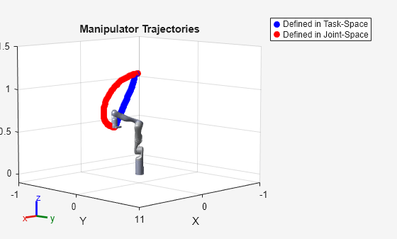
Visualize the task-space trajectory. Iterate through the stateTask states and interpolate based on the current time.
for i=1:length(trajTimes)
    % Current time
    tNow= trajTimes(i);
    % Interpolate simulated joint positions to get configuration at current time
    configNow = interp1(tTask,stateTask(:,1:numJoints),tNow);
    poseNow = getTransform(robot,configNow,endEffector);
    show(robot,configNow,'PreservePlot',false,'Frames','off');
    taskSpaceMarker = plot3(poseNow(1,4),poseNow(2,4),poseNow(3,4),'b.','MarkerSize',20);
    drawnow;
end
Visualize the joint-space trajectory. Iterate through the jointTask states and interpolate based on the current time.
% Return to initial configuration
show(robot,currentRobotJConfig,'PreservePlot',false,'Frames','off');

for i=1:length(trajTimes)
    % Current time
    tNow= trajTimes(i);
    % Interpolate simulated joint positions to get configuration at current time
    configNow = interp1(tJoint,stateJoint(:,1:numJoints),tNow);
    poseNow = getTransform(robot,configNow,endEffector);
    show(robot,configNow,'PreservePlot',false,'Frames','off');
    jointSpaceMarker = plot3(poseNow(1,4),poseNow(2,4),poseNow(3,4),'r.','MarkerSize',20);
    drawnow;
end

% Add a legend and title
legend([taskSpaceMarker jointSpaceMarker], {'Defined in Task-Space', 'Defined in Joint-Space'});
title('Manipulator Trajectories')

See Also
taskSpaceMotionModel | jointSpaceMotionModel | inverseKinematics