sgolay

Savitzky-Golay filter design

Syntax

b = sgolay(m,fl)

b = sgolay(m,fl,w)

[b,g] = sgolay(___)

Description

b = sgolay(m,fl) designs a Savitzky-Golay FIR smoothing filter with polynomial order m and frame length fl.

b = sgolay(m,fl,w) specifies a weighting vector, w, which contains the real, positive-valued weights to be used during the least-squares minimization.

[b,g] = sgolay(___) returns the matrix g of differentiation filters. You can use these output arguments with any of the previous input syntaxes.

Examples

Savitzky-Golay Smoothing of Noisy Sinusoid

Generate a signal that consists of a 0.2 Hz sinusoid embedded in white Gaussian noise and sampled five times a second for 200 seconds.

dt = 1/5;
t = (0:dt:200-dt)';

x = 5*sin(2*pi*0.2*t) + randn(size(t));

Use sgolay to smooth the signal. Use 21-sample frames and fourth order polynomials.

order = 4;
framelen = 21;

b = sgolay(order,framelen);

Compute the steady-state portion of the signal by convolving it with the center row of b.

ycenter = conv(x,b((framelen+1)/2,:),'valid');

Compute the transients. Use the last rows of b for the startup and the first rows of b for the terminal.

ybegin = b(end:-1:(framelen+3)/2,:) * x(framelen:-1:1);
yend = b((framelen-1)/2:-1:1,:) * x(end:-1:end-(framelen-1));

Concatenate the transients and the steady-state portion to generate the complete smoothed signal. Plot the original signal and the Savitzky-Golay estimate.

y = [ybegin; ycenter; yend];
plot([x y])
legend('Noisy Sinusoid','S-G smoothed sinusoid')

Savitzky-Golay Filter with Weights

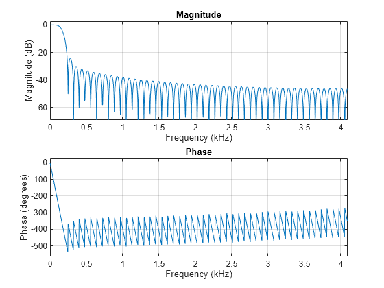
Design a Savitzky-Golay smoothing filter with 5th-order polynomials to filter a noisy signal sampled at ${\mathit{F}}_{\mathit{s}}=8192$ Hz. Use a Hamming window. The frame length is 101 samples.

Fs = 8192;
m = 5;
fl = 101;

weights = hamming(fl);

b = sgolay(m,fl,weights);

Plot the frequency response for the center row of b. Use 1024 FFT points.

NFFT = 1024;
freqz(b((fl+1)/2,:),1,NFFT,Fs)

For more information about weighing vectors and the impact on signal filtering performance, see Design and Analyze Savitzky-Golay Filters.

Savitzky-Golay Differentiation

Generate a signal that consists of a 0.2 Hz sinusoid embedded in white Gaussian noise and sampled four times a second for 20 seconds.

dt = 0.25;
t = (0:dt:20-1)';

x = 5*sin(2*pi*0.2*t)+0.5*randn(size(t));

Estimate the first three derivatives of the sinusoid using the Savitzky-Golay method. Use 25-sample frames and fifth order polynomials. Divide the columns by powers of dt to scale the derivatives correctly.

[b,g] = sgolay(5,25);

dx = zeros(length(x),4);
for p = 0:3
  dx(:,p+1) = conv(x, factorial(p)/(-dt)^p * g(:,p+1), 'same');
end

Plot the original signal, the smoothed sequence, and the derivative estimates.

plot(x,'.-')
hold on
plot(dx)
hold off

legend('x','x (smoothed)','x''','x''''', 'x''''''')
title('Savitzky-Golay Derivative Estimates')

Input Arguments

m — Polynomial order

nonnegative integer

Polynomial order, specified as a nonnegative integer. The value of m must be smaller than fl. If m = fl – 1, then the designed filter produces no smoothing.

fl — Frame length

positive odd integer

Frame length, specified as a positive odd integer. The value of fl must be greater than m.

w — Weighting vector

ones(fl,1) (default) | real positive vector

Weighting vector, specified as a real positive vector. The weighting vector has the same length as fl and is used to perform least-squares minimization.

Output Arguments

b — Time-varying FIR filter coefficients

matrix

Time-varying FIR filter coefficients, specified as a fl-by-fl matrix. In a smoothing filter implementation (for example, sgolayfilt), the last (fl-1)/2 rows (each an FIR filter) are applied to the signal during the startup transient, and the first (fl-1)/2 rows are applied to the signal during the terminal transient. The center row is applied to the signal in the steady state.

g — Matrix of differentiation filters

matrix

Matrix of differentiation filters, specified as a matrix. Each column of g is a differentiation filter for derivatives of order p-1, where p is the column index. Given a signal x of length fl, you can find an estimate of the p^th order derivative, xp, of its middle value from xp((fl+1)/2) = (factorial(p)) * g(:,p+1)' * x.

Algorithms

Savitzky-Golay filters are used to smooth out noisy signals with a large frequency span. Savitzky-Golay smoothing filters tend to filter out less of the signal's high-frequency content than standard averaging FIR filters. However, they are less successful at rejecting noise when noise levels are particularly high.

In general, filtering consists of replacing each point of a signal by some combination of the signal values contained in a moving window centered at the point, on the assumption that nearby points measure nearly the same underlying value. For example, moving average filters replace each data point with the local average of the surrounding data points. If a given data point has k points to the left and k points to the right, for a total window length of L = 2k + 1, the moving average filter makes the replacement

$$x_s\to {\widehat{x}}_s=\frac{1}{L}{\displaystyle \sum _{r=-k}^k{x}_{s+r}.}$$

Savitzky-Golay filters generalize this idea by least-squares fitting an nth-order polynomial through the signal values in the window and taking the calculated central point of the fitted polynomial curve as the new smoothed data point. For a given point, x_s,

$$\left[\begin{array}{c}{x}_{s-k}\\ ⋮\\ x_{s-1}\\ x_s\\ x_{s+1}\\ ⋮\\ x_{s+k}\end{array}\right]=\left[\begin{array}{c}{b}_0+b_1\left(t_s-k\Delta t\right)+b_2{\left(t_s-k\Delta t\right)}^2+\cdots +b_n{\left(t_s-k\Delta t\right)}^n\\ ⋮\\ b_0+b_1\left(t_s-1\Delta t\right)+b_2{\left(t_s-1\Delta t\right)}^2+\cdots +b_n{\left(t_s-1\Delta t\right)}^n\\ b_0+b_1\left(t_s-0\Delta t\right)+b_2{\left(t_s-0\Delta t\right)}^2+\cdots +b_n{\left(t_s-0\Delta t\right)}^n\\ b_0+b_1\left(t_s+1\Delta t\right)+b_2{\left(t_s+1\Delta t\right)}^2+\cdots +b_n{\left(t_s+1\Delta t\right)}^n\\ ⋮\\ b_0+b_1\left(t_s+k\Delta t\right)+b_2{\left(t_s+k\Delta t\right)}^2+\cdots +b_n{\left(t_s+k\Delta t\right)}^n\end{array}\right]=\left[\begin{array}{c}{a}_0+a_1\left(-k\right)+a_2{\left(-k\right)}^2+\cdots +a_n{\left(-k\right)}^n\\ ⋮\\ a_0+a_1\left(-1\right)+a_2{\left(-1\right)}^2+\cdots +a_n{\left(-1\right)}^n\\ a_0+a_1\left(0\right)+a_2{\left(0\right)}^2+\cdots +a_n{\left(0\right)}^n\\ a_0+a_1\left(1\right)+a_2{\left(1\right)}^2+\cdots +a_n{\left(1\right)}^n\\ ⋮\\ a_0+a_1\left(k\right)+a_2{\left(k\right)}^2+\cdots +a_n{\left(k\right)}^n\end{array}\right]$$

or, in terms of matrices,

$$x=\left[\begin{array}{ccccc}1& -k& {\left(-k\right)}^2& \cdots & {\left(-k\right)}^n\\ ⋮& ⋮& ⋮& ⋰& ⋮\\ 1& -2& {\left(-2\right)}^2& \cdots & {\left(-2\right)}^n\\ 1& -1& {\left(-1\right)}^2& \cdots & {\left(-1\right)}^n\\ 1& 0& 0& \cdots & 0\\ 1& 1& 1^2& \cdots & 1^n\\ 1& 2& 2^2& \cdots & 2^n\\ ⋮& ⋮& ⋮& \ddots & ⋮\\ 1& k& k^2& \cdots & k^n\end{array}\right]\left[\begin{array}{c}{a}_0\\ ⋮\\ a_n\end{array}\right]\equiv Ha.$$

To find the Savitzky-Golay estimates, use the pseudoinverse of H to compute a and then premultiply by H:

$$\widehat{x}=H{\left(H^{T}H\right)}^{-1}{H}^{T}x=Bx.$$

To avoid ill-conditioning, sgolay uses the qr function to compute an economy-size decomposition of H as H = QR, in terms of which B = QQ^T.

It is necessary to compute B only once. The Savitzky-Golay estimates for most signal points result from convolving the signal with the center row of B. The result is the steady-state portion of the filtered signal. The first k rows of B yield the initial transient, and the final k rows of B yield the final transient. See sgolayfilt for an example. It is possible to improve noise suppression by increasing the window length, but this introduces ringing analogous to the Gibbs phenomenon near any transients.

References

[1] Orfanidis, Sophocles J. Introduction to Signal Processing. Englewood Cliffs, NJ: Prentice Hall, 1996.

[2] Press, William H., Saul A. Teukolsky, William T. Vetterling, and Brian P. Flannery. Numerical Recipes in C: The Art of Scientific Computing. New York: Cambridge University Press, 1992.

[3] Schafer, Ronald W. “What Is a Savitzky-Golay Filter? [Lecture Notes].” IEEE Signal Processing Magazine Vol. 28, Number 4, July 2011, pp. 111–117. https://doi.org/10.1109/MSP.2011.941097.

Extended Capabilities

C/C++ Code Generation
Generate C and C++ code using MATLAB® Coder™.

Version History

Introduced before R2006a