Frequency-Domain Linear Regression
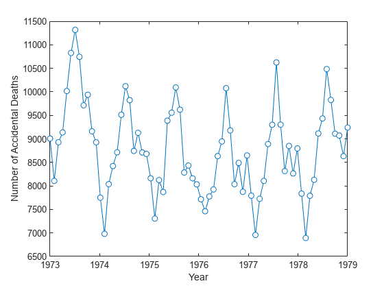
This example shows how to use the discrete Fourier transform to construct a linear regression model for a time series. The time series used in this example is the monthly number of accidental deaths in the United States from 1973 to 1979. The data are published in Brockwell and Davis (2006). The original source is the U. S. National Safety Council.
Enter the data. Copy the exdata matrix into the MATLAB® workspace.
exdata = [
        9007       7750       8162       7717       7792       7836
        8106       6981       7306       7461       6957       6892
        8928       8038       8124       7776       7726       7791
        9137       8422       7870       7925       8106       8129
       10017       8714       9387       8634       8890       9115
       10826       9512       9556       8945       9299       9434
       11317      10120      10093      10078      10625      10484
       10744       9823       9620       9179       9302       9827
        9713       8743       8285       8037       8314       9110
        9938       9129       8433       8488       8850       9070
        9161       8710       8160       7874       8265       8633
        8927       8680       8034       8647       8796       9240];
exdata is a 12-by-6 matrix. Each column of exdata contains 12 months of data. The first row of each column contains the number of US accidental deaths for January of the corresponding year. The last row of each column contains the number of US accidental deaths for December of the corresponding year.
Reshape the data matrix into a 72-by-1 time series and plot the data for the years 1973 to 1978.
ts = reshape(exdata,72,1);
years = linspace(1973,1979,72);

plot(years,ts,"o-",MarkerFaceColor="auto")
xlabel("Year")
ylabel("Number of Accidental Deaths")

A visual inspection of the data indicates that number of accidental deaths varies in a periodic manner. The period of the oscillation appears to be roughly 1 year (12 months). The periodic nature of the data suggests that an appropriate model may be
where is the overall mean, is the length of the time series, and is a white noise sequence of independent and identically-distributed (IID) Gaussian random variables with zero mean and some variance. The additive noise term accounts for the randomness inherent in the data. The parameters of the model are the overall mean and the amplitudes of the cosines and sines. The model is linear in the parameters.
To construct a linear regression model in the time domain, you have to specify which frequencies to use for the cosines and sines, form the design matrix, and solve the normal equations in order to obtain the least-squares estimates of the model parameters. In this case, it is easier to use the discrete Fourier transform to detect the periodicities, retain only a subset of the Fourier coefficients, and invert the transform to obtain the fitted time series.
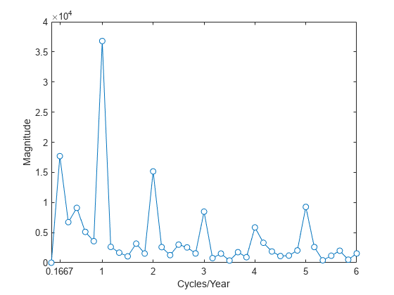
Perform a spectral analysis of the data to reveal which frequencies contribute significantly to the variability in the data. Because the overall mean of the signal is approximately 9,000 and is proportional to the Fourier transform at 0 frequency, subtract the mean prior to the spectral analysis. This reduces the large magnitude Fourier coefficient at 0 frequency and makes any significant oscillations easier to detect. The frequencies in the Fourier transform are spaced at an interval that is the reciprocal of the time series length, 1/72. Sampling the data monthly, the highest frequency in the spectral analysis is 1 cycle/2 months. In this case, it is convenient to look at the spectral analysis in terms of cycles/year so scale the frequencies accordingly for visualization.
tsdft = fft(ts-mean(ts));
freq = 0:1/72:1/2;

plot(freq.*12,abs(tsdft(1:length(ts)/2+1)),"o-", ...
    MarkerFaceColor="auto")
xlabel("Cycles/Year")
ylabel("Magnitude")
ax = gca;
ax.XTick = [1/6 1 2 3 4 5 6];

Based on the magnitudes, the frequency of 1 cycle/12 months is the most significant oscillation in the data. The magnitude at 1 cycle/12 months is more than twice as large as any other magnitude. However, the spectral analysis reveals that there are also other periodic components in the data. For example, there appears to be periodic components at harmonics (integer multiples) of 1 cycle/12 months. There also appears to be a periodic component with a period of 1 cycle/72 months.
Based on the spectral analysis of the data, fit a simple linear regression model using a cosine and sine term with a frequency of the most significant component: 1 cycle/year (1 cycle/12 months).
Determine the frequency bin in the discrete Fourier transform that corresponds to 1 cycle/12 months. Because the frequencies are spaced at 1/72 and the first bin corresponds to 0 frequency, the correct bin is 72/12+1. This is the frequency bin of the positive frequency. You must also include the frequency bin corresponding to the negative frequency: -1 cycle/12 months. With MATLAB indexing, the frequency bin of the negative frequency is 72-72/12+1.
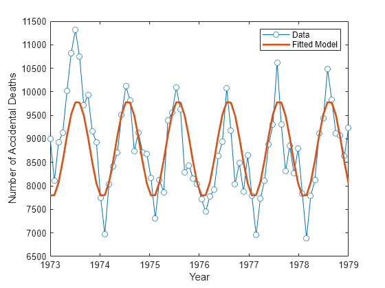
Create a 72-by-1 vector of zeros. Fill the appropriate elements of the vector with the Fourier coefficients corresponding to a positive and negative frequency of 1 cycle/12 months. Invert the Fourier transform and add the overall mean to obtain a fit to the accidental death data.
freqbin = 72/12;
freqbins = [freqbin 72-freqbin]+1;
tsfit = zeros(72,1);
tsfit(freqbins) = tsdft(freqbins);
tsfit = ifft(tsfit);
mu = mean(ts);
tsfit = mu+tsfit;
Plot the original data along with the fitted series using two Fourier coefficients.
plot(years,ts,"o-",MarkerFaceColor="auto")
xlabel("Year")
ylabel("Number of Accidental Deaths")
hold on
plot(years,tsfit,LineWidth=2)
legend("Data","Fitted Model")
hold off

The fitted model appears to capture the general periodic nature of the data and supports the initial conclusion that data oscillate with a cycle of 1 year.
To assess how adequately the single frequency of 1 cycle/12 months accounts for the observed time series, form the residuals. If the residuals resemble a white noise sequence, the simple linear model with one frequency has adequately modeled the time series.
To assess the residuals, use the autocorrelation sequence with 95%-confidence intervals for a white noise.
resid = ts-tsfit;
[xc,lags] = xcorr(resid,50,"coeff");

stem(lags(51:end),xc(51:end),"filled")
hold on
lconf = -1.96*ones(51,1)/sqrt(72);
uconf = 1.96*ones(51,1)/sqrt(72);
plot(lags(51:end),lconf,"r")
plot(lags(51:end),uconf,"r")
xlabel("Lag")
ylabel("Correlation Coefficient")
title("Autocorrelation of Residuals")
hold off

The autocorrelation values fall outside the 95% confidence bounds at a number of lags. It does not appear that the residuals are white noise. The conclusion is that the simple linear model with one sinusoidal component does not account for all the oscillations in the number of accidental deaths. This is expected because the spectral analysis revealed additional periodic components in addition to the dominant oscillation. Creating a model that incorporates additional periodic terms indicated by the spectral analysis will improve the fit and whiten the residuals.
Fit a model which consists of the three largest Fourier coefficient magnitudes. Because you have to retain the Fourier coefficients corresponding to both negative and positive frequencies, retain the largest 6 indices.
tsfit2dft = zeros(72,1);
[Y,I] = sort(abs(tsdft),"descend");
indices = I(1:6);
tsfit2dft(indices) = tsdft(indices);
Demonstrate that preserving only 6 of the 72 Fourier coefficients (3 frequencies) retains most of the signal's energy. First, demonstrate that retaining all the Fourier coefficients yields energy equivalence between the original signal and the Fourier transform.
norm(1/sqrt(72)*tsdft,2)/norm(ts-mean(ts),2)
ans =
1.0000
The ratio is 1. Now, examine the energy ratio where only 3 frequencies are retained.
norm(1/sqrt(72)*tsfit2dft,2)/norm(ts-mean(ts),2)
ans =
0.8991
Almost 90% of the energy is retained. Equivalently, 90% of the variance of the time series is accounted for by 3 frequency components.
Form an estimate of the data based on 3 frequency components. Compare the original data, the model with one frequency, and the model with 3 frequencies.
tsfit2 = mu+ifft(tsfit2dft,"symmetric");

plot(years,ts,"o-",MarkerFaceColor="auto")
xlabel("Year")
ylabel("Number of Accidental Deaths")
hold on
plot(years,tsfit,LineWidth=2)
plot(years,tsfit2,LineWidth=2)
legend("Data","1 Frequency","3 Frequencies")
hold off

Using 3 frequencies has improved the fit to the original signal. You can see this by examining the autocorrelation of the residuals from the 3-frequency model.
resid = ts-tsfit2;
[xc,lags] = xcorr(resid,50,"coeff");

stem(lags(51:end),xc(51:end),"filled")
hold on
lconf = -1.96*ones(51,1)/sqrt(72);
uconf = 1.96*ones(51,1)/sqrt(72);
plot(lags(51:end),lconf,"r")
plot(lags(51:end),uconf,"r")
xlabel("Lag")
ylabel("Correlation Coefficient")
title("Autocorrelation of Residuals")
hold off

Using 3 frequencies has resulted in residuals that more closely approximate a white noise process.
Demonstrate that the parameter values obtained from the Fourier transform are equivalent to a time-domain linear regression model. Find the least-squares estimates for the overall mean, the cosine amplitudes, and the sine amplitudes for the three frequencies by forming the design matrix and solving the normal equations. Compare the fitted time series with that obtained from the Fourier transform.
X = ones(72,7);
X(:,2) = cos(2*pi/72*(0:71))';
X(:,3) = sin(2*pi/72*(0:71))';
X(:,4) = cos(2*pi*6/72*(0:71))';
X(:,5) = sin(2*pi*6/72*(0:71))';
X(:,6) = cos(2*pi*12/72*(0:71))';
X(:,7) = sin(2*pi*12/72*(0:71))';
beta = X\ts;
tsfit_lm = X*beta;
max(abs(tsfit_lm-tsfit2))
ans =
7.2760e-12
The two methods yield identical results. The maximum absolute value of the difference between the two waveforms is on the order of 10-12. In this case, the frequency-domain approach was easier than the equivalent time-domain approach. You naturally use a spectral analysis to visually inspect which oscillations are present in the data. From that step, it is simple to use the Fourier coefficients to construct a model for the signal consisting of a sum cosines and sines.
For more details on spectral analysis in time series and the equivalence with time-domain regression see (Shumway and Stoffer, 2006).
While spectral analysis can answer which periodic components contribute significantly to the variability of the data, it does not explain why those components are present. If you examine these data closely, you see that the minimum values in the 12-month cycle tend to occur in February, while the maximum values occur in July. A plausible explanation for these data is that people are naturally more active in summer than in the winter. Unfortunately, as a result of this increased activity, there is an increased probability of the occurrence of fatal accidents.
References
Brockwell, Peter J., and Richard A. Davis. Time Series: Theory and Methods. New York: Springer, 2006.
Shumway, Robert H., and David S. Stoffer. Time Series Analysis and Its Applications with R Examples. New York: Springer, 2006.