CovariateModel
Define relationship between parameters and covariates
Description
A CovariateModel object defines the relationship between
estimated parameters and covariates.
Use a CovariateModel object as an input argument to sbiofitmixed to fit a model with covariate dependencies. Before using the
CovariateModel object, set the FixedEffectValues
property to specify the initial estimates for the fixed effects.
Creation
Description
Input Arguments
Properties
Object Functions
constructDefaultFixedEffectValues | Create structure containing initial estimates fixed effects needed for fit |
verify | Check covariate model for errors |
Examples
Create an empty CovariateModel object.
covModel = CovariateModel;
Set its Expression property to define the relationships between parameters (Cl, V, and k) and covariate (w). You must use theta as a prefix for all fixed effects and eta for random effects.
covModel.Expression = ["Cl = theta1 + theta2*w + eta1","V = theta3 + eta2","k = theta4 + eta3"];
Display the names of fixed effects.
covModel.FixedEffectNames
ans = 4×1 cell
    {'theta1'}
    {'theta3'}
    {'theta4'}
    {'theta2'}
The FixedEffectDescription property displays which fixed effects correspond to which parameter. For instance, theta1 is the fixed effect for the Cl parameter, and theta2 is the fixed effect for the weight covariate that has a correlation with Cl parameter, denoted as Cl/w.
covModel.FixedEffectDescription
ans = 4×1 cell
    {'Cl'  }
    {'V'   }
    {'k'   }
    {'Cl/w'}
Specify initial estimates for the fixed effects. Create a default structure containing initial estimates using the constructDefaultFixedEffectValues function.
initialEstimates = constructDefaultFixedEffectValues(covModel)
initialEstimates = struct with fields:
    theta1: 0
    theta3: 0
    theta4: 0
    theta2: 0
Update the initial estimate value of each fixed effects.
initialEstimates.theta1 = 1.20;
initialEstimates.theta2 = 0.30;
initialEstimates.theta3 = 0.90;
initialEstimates.theta4 = 0.10;
Update the FixedEffectValues property to use the updated initial estimates.
covModel.FixedEffectValues = initialEstimates;
Check the covariate model for errors.
verify(covModel)
Estimate nonlinear mixed-effects parameters using clinical pharmacokinetic data collected from 59 infants. Evaluate the fitted model given new data or dosing information.
Load Data
This example uses data collected on 59 preterm infants given phenobarbital during the first 16 days after birth [1]. ds is a table containing the concentration-time profile data and covariate information for each infant (or group).
load pheno.mat ds
Convert to groupedData
Convert the data to the groupedData format for parameter estimation.
data = groupedData(ds);
Display the first few rows of data.
data(1:5,:)
ans =

  5×6 groupedData

    ID    TIME    DOSE    WEIGHT    APGAR    CONC
    __    ____    ____    ______    _____    ____

    1        0     25      1.4        7       NaN
    1        2    NaN      1.4        7      17.3
    1     12.5    3.5      1.4        7       NaN
    1     24.5    3.5      1.4        7       NaN
    1       37    3.5      1.4        7       NaN
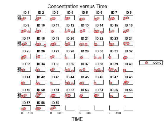
Visualize Data
Display the data in a trellis plot.
t = sbiotrellis(data, 'ID', 'TIME', 'CONC', 'marker', 'o',...
       'markerfacecolor', [.7 .7 .7], 'markeredgecolor', 'r', ...
       'linestyle', 'none');
t.plottitle = 'Concentration versus Time';
Create a One-Compartment PK Model
Create a simple one-compartment PK model, with bolus dose administration and linear clearance elimination, to fit the data.
pkmd = PKModelDesign;
addCompartment(pkmd,'Central','DosingType','Bolus',...
                    'EliminationType','linear-clearance',...
                    'HasResponseVariable',true,'HasLag',false);
onecomp = pkmd.construct;
Map model species to response data.
responseMap = 'Drug_Central = CONC';Define Estimated Parameters
The parameters to estimate in this model are the volume of the central compartment (Central) and the clearance rate (Cl_Central). sbiofitmixed calculates fixed and random effects for each parameter. The underlying algorithm computes normally distributed random effects, which might violate constraints for biological parameters that are always positive, such as volume and clearance. Therefore, specify a transform for the estimated parameters so that the transformed parameters follow a normal distribution. The resulting model is
and
where , , and are the fixed effects, random effects, and estimated parameter values respectively, calculated for each infant (group) . Some arbitrary initial estimates for V (volume of central compartment) and Cl (clearance rate) are used here in the absence of better empirical data.
estimatedParams = estimatedInfo({'log(Central)','log(Cl_Central)'},'InitialValue',[1 1]);Define Dosing
All infants were given the drug, represented by the Drug_Central species, where the dosing schedule varies among infants. The amount of drug is listed in the data variable DOSE. You can automatically generate dose objects from the data and use them during fitting. In this example, Drug_Central is the target species that receives the dose.
sampleDose = sbiodose('sample','TargetName','Drug_Central');
doses = createDoses(data,'DOSE','',sampleDose);
Fit the Model
Use sbiofitmixed to fit the one-compartment model to the data.
nlmeResults = sbiofitmixed(onecomp,data,responseMap,estimatedParams,doses,'nlmefit');Visualize Results
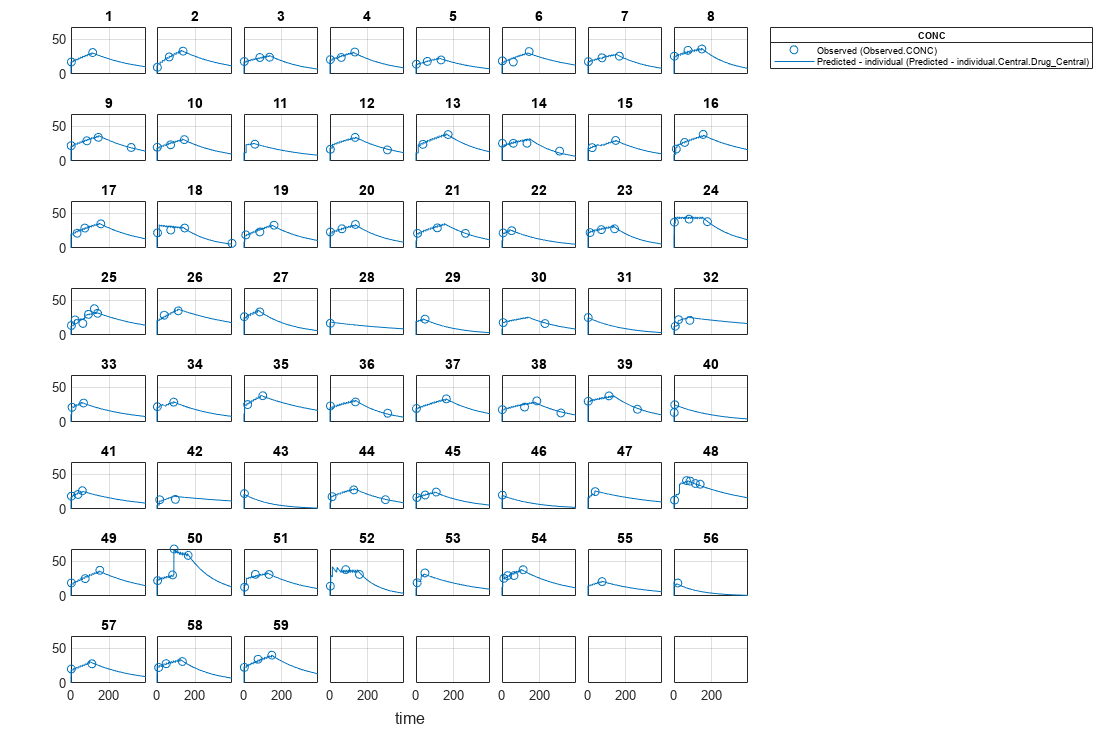
Visualize the fitted results using individual-specific parameter estimates.
plot(nlmeResults,'ParameterType','individual');
Use New Dosing Data to Simulate the Fitted Model
Suppose you want to predict how infants 1 and 2 would have responded under different dosing amounts. You can predict their responses as follows.
Create new dose objects with new dose amounts.
dose1 = doses(1);
dose1.Amount = dose1.Amount*2;
dose2 = doses(2);
dose2.Amount = dose2.Amount*1.5;
Use the predict function to evaluate the fitted model using the new dosing data. If you want response predictions at particular times, provide the new output time vector. Use the 'ParameterType' option to specify individual or population parameters to use. By default, predict uses the population parameters when you specify output times.
timeVec = [0:25:400];
newResults = predict(nlmeResults,timeVec,[dose1;dose2],'ParameterType','population');
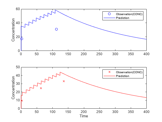
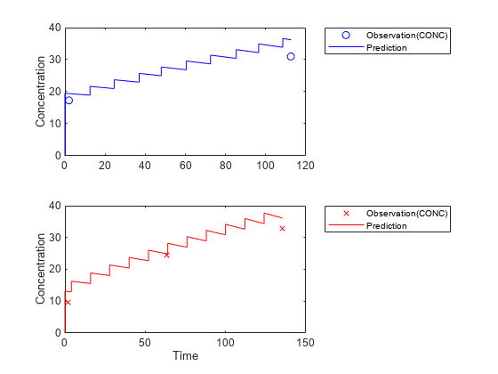
Visualize the predicted responses while overlapping the experimental data for infants 1 and 2.
figure;
subplot(2,1,1)
plot(data.TIME(data.ID == 1),data.CONC(data.ID == 1),'bo')
hold on
plot(newResults(1).Time,newResults(1).Data,'b')
hold off
ylabel('Concentration')
legend('Observation(CONC)','Prediction')
subplot(2,1,2)
plot(data.TIME(data.ID == 2),data.CONC(data.ID == 2),'rx')
hold on
plot(newResults(2).Time,newResults(2).Data,'r')
hold off
legend('Observation(CONC)','Prediction')
ylabel('Concentration')
xlabel('Time')
Create a Covariate Model for the Covariate Dependencies
Suppose there is a correlation between volume and weight, and possibly volume and APGAR score. Consider the effect of weight by modeling two of these covariate dependencies: the volume of central (Central) and the clearance rate (Cl_Central) vary with weight. The model becomes
and
Use the CovariateModel object to define the covariate dependencies. For details, see Specify a Covariate Model.
covModel = CovariateModel;
covModel.Expression = ({'Central = exp(theta1 + theta2*WEIGHT + eta1)',...
                        'Cl_Central = exp(theta3 + theta4*WEIGHT + eta2)'});
Use constructDefaultInitialEstimate to create an initialEstimates struct.
initialEstimates = covModel.constructDefaultFixedEffectValues;
Use the FixedEffectNames property to display the thetas (fixed effects) defined in the model.
covModel.FixedEffectNames
ans = 4×1 cell
    {'theta1'}
    {'theta3'}
    {'theta2'}
    {'theta4'}
Use the FixedEffectDescription property to show the descriptions of corresponding fixed effects (thetas) used in the covariate expression. For example, theta2 is the fixed effect for the weight covariate that correlates with the volume (Central), denoted as 'Central/WEIGHT'.
disp('Fixed Effects Description:');Fixed Effects Description:
disp(covModel.FixedEffectDescription);
    {'Central'          }
    {'Cl_Central'       }
    {'Central/WEIGHT'   }
    {'Cl_Central/WEIGHT'}
Set the initial guesses for the fixed-effect parameter values for Central and Cl_Central using the values estimated from fitting the base model.
initialEstimates.theta1 = nlmeResults.FixedEffects.Estimate(1);
initialEstimates.theta3 = nlmeResults.FixedEffects.Estimate(2);
covModel.FixedEffectValues = initialEstimates;
Fit the Model
nlmeResults_cov = sbiofitmixed(onecomp,data,responseMap,covModel,doses,'nlmefit');Display Fitted Parameters and Covariances
disp('Estimated Fixed Effects:');Estimated Fixed Effects:
disp(nlmeResults_cov.FixedEffects);
       Name            Description         Estimate    StandardError     RSE
    __________    _____________________    ________    _____________    ______

    {'theta1'}    {'Central'          }    -0.45664      0.078933       17.286
    {'theta3'}    {'Cl_Central'       }     -5.9519        0.1177       1.9775
    {'theta2'}    {'Central/WEIGHT'   }     0.52948      0.047342       8.9412
    {'theta4'}    {'Cl_Central/WEIGHT'}     0.61954      0.071386       11.522
disp('Estimated Covariance Matrix:');Estimated Covariance Matrix:
disp(nlmeResults_cov.RandomEffectCovarianceMatrix);
              eta1        eta2
            ________    ________

    eta1    0.046503           0
    eta2           0    0.041609
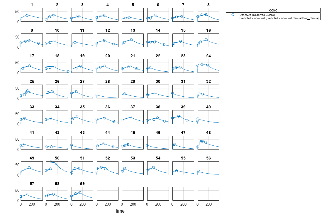
Visualize Results
Visualize the fitted results using individual-specific parameter estimates.
plot(nlmeResults_cov,'ParameterType','individual');
Use New Covariate Data to Evaluate the Fitted Model
Suppose you want to explore the responses of infants 1 and 2 using different covariate data, namely WEIGHT. You can do this by specifying the new WEIGHT data. The ID variable of the data corresponds to individual infants.
newData = data(data.ID == 1 | data.ID == 2,:);
newData.WEIGHT(newData.ID == 1) = 1.3;
newData.WEIGHT(newData.ID == 2) = 1.4;
Simulate the responses of infants 1 and 2 using the new covariate data.
[newResults_cov, newEstimates] = predict(nlmeResults_cov,newData,[dose1;dose2]);
newEstimates contains the updated parameter estimates for each individual (infants 1 and 2) after the model is reevaluated using the new covariate data.
newEstimates
newEstimates=4×3 table
    Group         Name         Estimate
    _____    ______________    _________

      1      {'Central'   }       2.5596
      1      {'Cl_Central'}    0.0065965
      2      {'Central'   }       1.7123
      2      {'Cl_Central'}    0.0064806
Compare to the estimated values from the original fit using the old covariate data.
nlmeResults_cov.IndividualParameterEstimates( ...
            nlmeResults_cov.IndividualParameterEstimates.Group == '1' | ...
            nlmeResults_cov.IndividualParameterEstimates.Group == '2',:)
ans=4×3 table
    Group         Name         Estimate
    _____    ______________    _________

      1      {'Central'   }       2.6988
      1      {'Cl_Central'}    0.0070181
      2      {'Central'   }       1.8054
      2      {'Cl_Central'}    0.0068948
Visualize the new simulation results together with the experimental data for infant 1 and 2.
figure;
subplot(2,1,1);
plot(data.TIME(data.ID == 1),data.CONC(data.ID == 1),'bo')
hold on
plot(newResults_cov(1).Time,newResults_cov(1).Data,'b')
hold off
ylabel('Concentration')
legend('Observation(CONC)','Prediction','Location','NorthEastOutside')
subplot(2,1,2)
plot(data.TIME(data.ID == 2),data.CONC(data.ID == 2),'rx')
hold on
plot(newResults_cov(2).Time,newResults_cov(2).Data,'r')
hold off
legend('Observation(CONC)','Prediction','Location','NorthEastOutside')
ylabel('Concentration')
xlabel('Time')
References
[1] Grasela, T. H. Jr., and S. M. Donn. "Neonatal population pharmacokinetics of phenobarbital derived from routine clinical data." Dev Pharmacol Ther 1985:8(6). 374-83.
This example uses data collected on 59 preterm infants given phenobarbital during the first 16 days after birth. Each infant received an initial dose followed by one or more sustaining doses by intravenous bolus administration. A total of between 1 and 6 concentration measurements were obtained from each infant at times other than dose times, for a total of 155 measurements. Infant weights and APGAR scores (a measure of newborn health) were also recorded. Data was described in [1], a study funded by the NIH/NIBIB grant P41-EB01975.
Load the data.
load pheno.mat ds
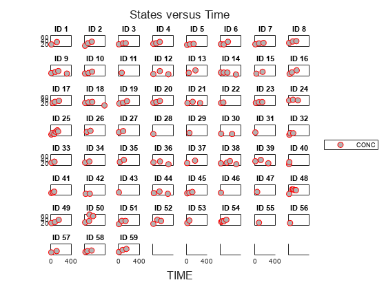
Visualize the data.
t = sbiotrellis(ds,'ID','TIME','CONC','marker','o','markerfacecolor',[.7 .7 .7],'markeredgecolor','r','linestyle','none');
t.plottitle = 'States versus Time';
Create a one-compartment PK model with bolus dosing and linear clearance to model such data.
pkmd = PKModelDesign;
pkmd.addCompartment('Central','DosingType','Bolus','EliminationType','linear-clearance',...
                    'HasResponseVariable',true,'HasLag',false);
onecomp = pkmd.construct;
Suppose there is a correlation between the volume of the central compartment (Central) and the weight of infants. You can define this parameter-covariate relationship using a covariate model that can be described as
,
where, for each ith infant, V is the volume, θs (thetas) are fixed effects, η (eta) represents random effects, and WEIGHT is the covariate.
covM = CovariateModel;
covM.Expression = {'Central = exp(theta1+theta2*WEIGHT+eta1)'};
Define the fixed and random effects. The column names of each table must have the names of fixed effects and random effects, respectively.
thetas = table(1.4,0.05,'VariableNames',{'theta1','theta2'});
eta1 = table(0.2,'VariableNames',{'eta1'});
Change the group label ID to GROUP as required by the sbiosampleparameters function.
ds.Properties.VariableNames{'ID'} = 'GROUP';Generate parameter values for the volumes of central compartments Central based on the covariate model for all infants in the data set.
phi = sbiosampleparameters(covM.Expression,thetas,eta1,ds);
You can then simulate the model using the sampled parameter values. For convenience, use the function-like interface provided by a SimFunction object.
First, construct a SimFunction object using the createSimFunction method, specifying the volume (Central) as the parameter, and the drug concentration in the compartment (Drug_Central) as the output of the SimFunction object, and the dosed species.
f = createSimFunction(onecomp,covM.ParameterNames,'Drug_Central','Drug_Central');
The data set ds contains dosing information for each infant, and the groupedData object provides a convenient way to extract such dosing information. Convert ds to a groupedData object and extract dosing information.
grpData = groupedData(ds);
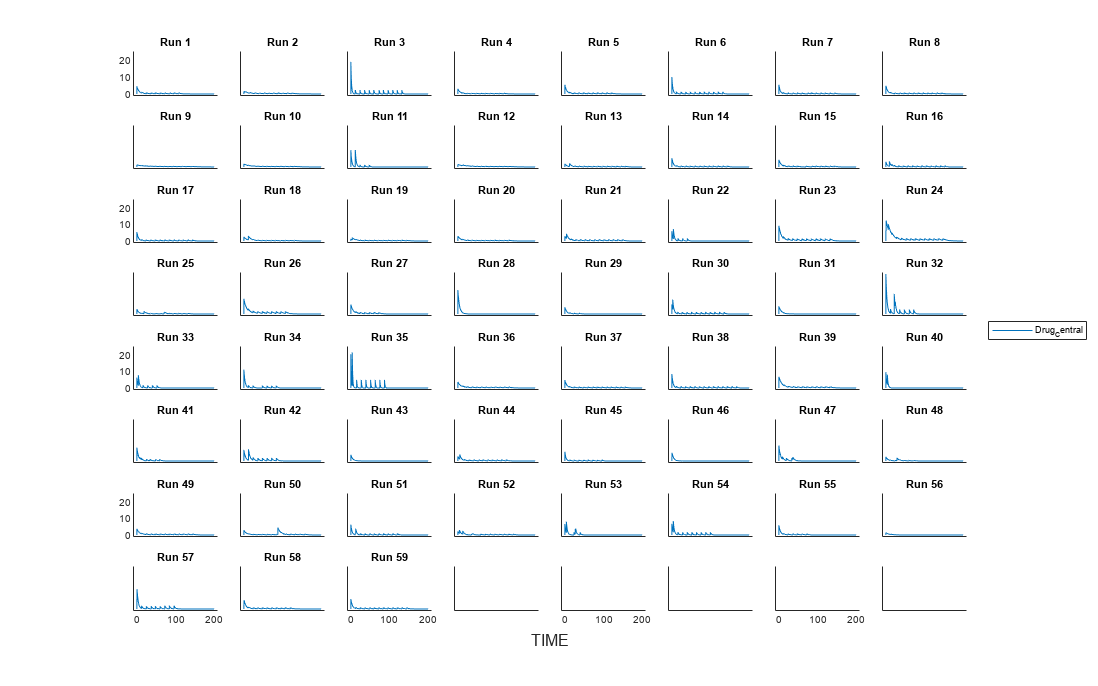
doses = createDoses(grpData,'DOSE');Simulate the model using the sampled parameter values from phi and the extracted dosing information of each infant, and plot the results. The ith run uses the ith parameter value in phi and dosing information of the ith infant.
t = sbiotrellis(f(phi,200,doses.getTable),[],'TIME','Drug_Central');
% Resize the figure.
t.hFig.Position(:) = [100 100 1280 800];
Version History
Introduced in R2011b