Suppress PMSM Harmonics Using Adaptive Notch Filter
This example shows how to reduce harmonic distortion in a permanent magnet synchronous machine (PMSM) using the Adaptive Notch Filter (ANF) block in Simulink® Control Design™. In numerous fields, including acoustics, motor control, and power systems, distortion is present. This distortion can take many forms and can be caused by multiple sources, but the most common form of distortion is harmonic distortion. No matter the type of distortion, it can have a negative affect on system performance such as impacting power delivery, vibration, or audible noise. Because of this, it is desired to reduce this distortion in order to improve system performance. One method to reduce harmonic distortion is known as an Adaptive Notch Filter (ANF). In this example, the Adaptive Notch Filter block in Simulink® Control Design™ is implemented to reduce harmonic distortion for a PMSM model.
Model Overview
The model used in this example is derived from the Motor Control Blockset™ example Determine Power Losses and THD for PWM Methods (Motor Control Blockset).The original example compares different PWM strategies and uses the total harmonic distortion metric to compare them. For this example, you use the first PWM strategy with distortion added to the plant.
Open the model.
scdAdaptiveFilterPMSMinit
             model: 'Teknic-2310P'
                sn: '003'
                 p: 4
                Rs: 0.3600
                Ld: 2.0000e-04
                Lq: 2.0000e-04
                 J: 7.0616e-06
                 B: 2.6369e-06
                Ke: 4.6400
                Kt: 0.0384
           I_rated: 7.1000
             N_max: 6000
    PositionOffset: 0.1712
          QEPSlits: 1000
            FluxPM: 0.0064
           T_rated: 0.2724
            N_base: 4107

               model: 'BoostXL-DRV8305'
                  sn: 'INV_XXXX'
                V_dc: 24
              I_trip: 10
              Rds_on: 0.0020
              Rshunt: 0.0070
       CtSensAOffset: 2295
       CtSensBOffset: 2286
       CtSensCOffset: 2295
             ADCGain: 1
         EnableLogic: 1
        invertingAmp: 1
          ISenseVref: 3.3000
    ISenseVoltPerAmp: 0.0700
           ISenseMax: 23.5714
             R_board: 0.0043
     CtSensOffsetMax: 2500
     CtSensOffsetMin: 1500

    V_base: 13.8564
    I_base: 23.5714
    N_base: 4107
    P_base: 489.9229
    T_base: 0.9045
mdl = "scdAdaptiveFilterHarmonicsPMSM";
open_system(mdl)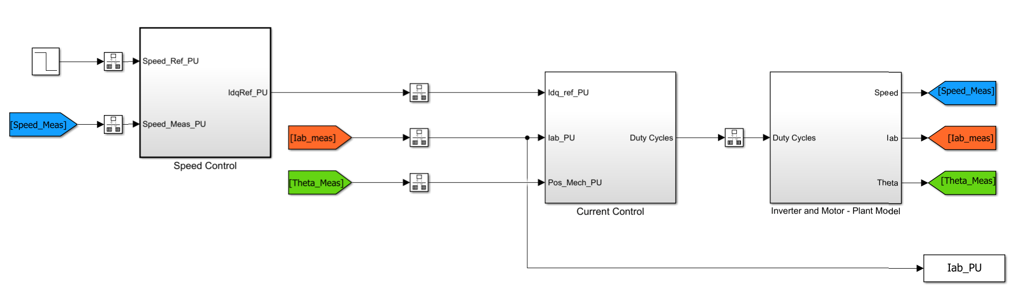
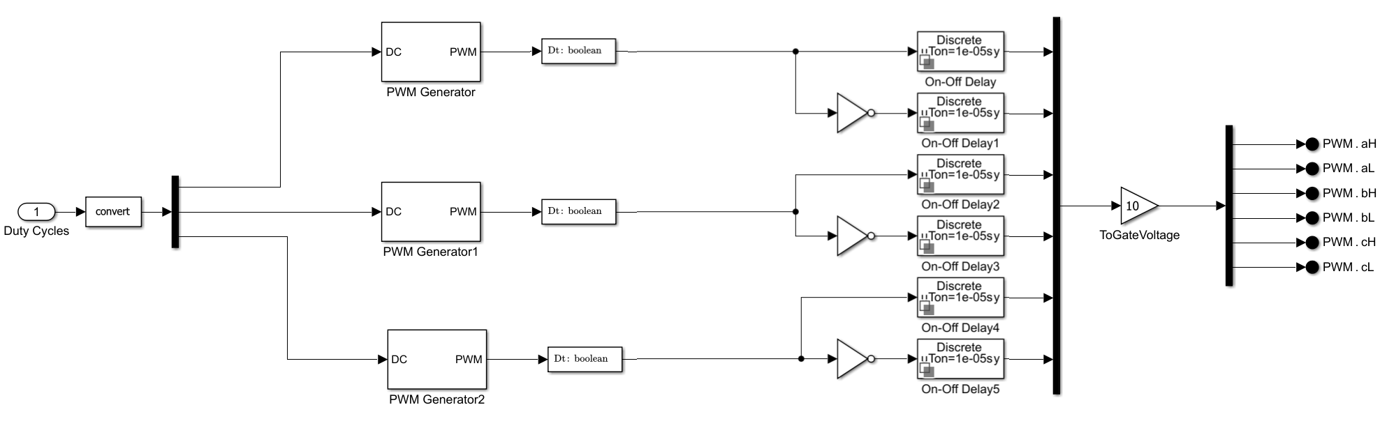
Adding in Harmonic Distortion
The baseline model does not contain any sources of distortion typically found in the real world such as magnetic saturation, motor winding asymmetry, dead time, and so on. To add distortion to the model, the example adds a delay time for enabling the IGBT switches to simulate dead-time. The higher this value of delay time, the more the distortion. This example uses a value of 10 microseconds which results in 5th and 7th harmonic distortion and a total harmonic distortion of almost 10%. The goal is to reduce these harmonics for various motor speeds and improve the total harmonic distortion.
Reducing 5th and 7th Harmonic Distortion in Synchronous Reference Frame
5th and 7th Harmonic in Synchronous Reference Frame
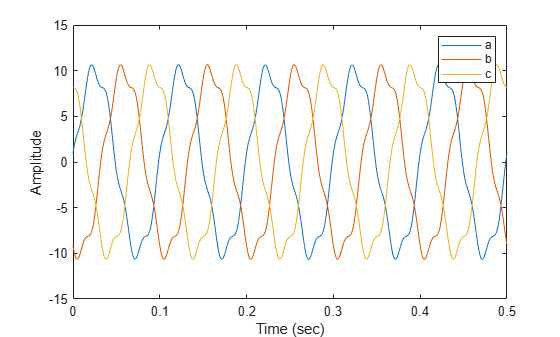
In the stator (stationary) reference frame, the distortion caused by dead-time results in a 5th and 7th harmonic. For field-oriented control, the current controllers act in the rotor (synchronous) reference frame. When transforming a three-phase signal from the stationary reference frame to the synchronous reference frame, all frequency components shift by the fundamental frequency. For example, if the fundamental frequency has an amplitude of 3 and a frequency of 10 rad/sec then, in the synchronous reference frame, this would result in a signal with an amplitude of 3 at a frequency of 0 rad/sec (or DC). The same applies to harmonics, that is, the 7th harmonic becomes the 6th harmonic. However, the 5th harmonic is negative sequence; meaning it rotates in an opposite direction from the fundamental, so it shifts to the 6th harmonic, instead of the 4th harmonic, in the synchronous reference frame. To show this, the examples first creates a three-phase waveform with a fundamental frequency of 10 Hz, and obtains a 5th harmonic and its FFT to use as a baseline.
w0 = 10*2*pi; % Fundamental Frequency
Ts = 1/10e3;
t = 0:Ts:0.5;

% Get 3-phase waveforms with 5th harmonic
yA = 10*sin(w0*t + 0) + cos(5*w0*t);
yB = 10*sin(w0*t - 2*pi/3) + cos(5*(w0*t-2*pi/3));
yC = 10*sin(w0*t + 2*pi/3) + cos(5*(w0*t+2*pi/3));
% Get FFT of Phase A
L = length(t);
Fs = 1/Ts;
fftA = fft(yA);

% Plot the 3-phase waveform
figure
plot(t,yA,t,yB,t,yC)
legend("a","b","c")
xlabel("Time (sec)")
ylabel("Amplitude")
Next, transform this three-phase set from the stationary reference frame to the synchronous reference frame using the Park transformation (for more information on this transformation see Clarke and Park Transforms). Also, take the FFT of the d-axis signal to compare to the stationary reference frame.
% Park Transform (ABC to DQ0)
theta = w0*t;
sinThetaA = sin(theta);
sinThetaB = sin(theta-2*pi/3);
sinThetaC = sin(theta+2*pi/3);
cosThetaA = cos(theta);
cosThetaB = cos(theta-2*pi/3);
cosThetaC = cos(theta+2*pi/3);
dq0 = zeros(3,length(theta));
for ii =1:length(theta)
 dq0(:,ii) = 2/3*[sinThetaA(ii) sinThetaB(ii) sinThetaC(ii);cosThetaA(ii) cosThetaB(ii) cosThetaC(ii); 0.5 0.5 0.5]*[yA(ii);yB(ii);yC(ii)];
end

% Get FFT of D-axis
fftD = fft(dq0(1,:));
In order to compare the waveforms, use the FFTs that were obtained previously and plot the magnitudes of the first 7 harmonics against each other using a bar graph.
% Plot Harmonics
idxPlot = ceil(w0/2/pi/(Fs/L)*(1:7));
figure
bar(1:7,[20*log10(abs(fftA(idxPlot))); 20*log10(abs(fftD(idxPlot)))])
xlabel("Harmonic Number");ylabel("Power (dB)");legend("Stationary","Synchronous")
title("Three Phase Harmonic Transformation for 5th Harmonic")
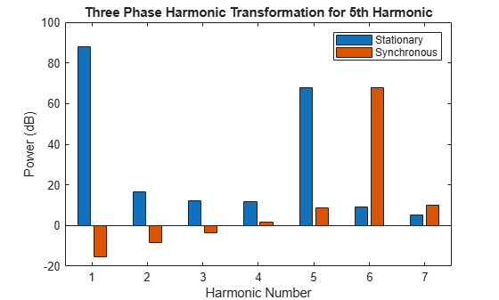
The stationary frame signal has large values at harmonics of 1 (the fundamental) and 5. The synchronous reference frame has a large value only at the 6th harmonic as the fundamental has moved to 0 and is not shown here. As expected, the 5th harmonic shifts, with the same magnitude, to the 6th harmonic in the synchronous reference frame. You can do the same for the 7th harmonic as the 5th harmonic. Create the 3-phase waveform with a 7th harmonic then transform to the synchronous reference frame. Take the FFTs of both phase A and the D-axis and plot using a bar graph.
% Get 3-phase waveforms with 5th harmonic
yA = 10*sin(w0*t + 0) + cos(7*w0*t);
yB = 10*sin(w0*t - 2*pi/3) + cos(7*(w0*t-2*pi/3));
yC = 10*sin(w0*t + 2*pi/3) + cos(7*(w0*t+2*pi/3));
% Get FFT of Phase A
L = length(t);
Fs = 1/Ts;
fftA = fft(yA);
% Park Transform (ABC to DQ0)
theta = w0*t;
sinThetaA = sin(theta);
sinThetaB = sin(theta-2*pi/3);
sinThetaC = sin(theta+2*pi/3);
cosThetaA = cos(theta);
cosThetaB = cos(theta-2*pi/3);
cosThetaC = cos(theta+2*pi/3);
dq0 = zeros(3,length(theta));
for ii =1:length(theta)
 dq0(:,ii) = 2/3*[sinThetaA(ii) sinThetaB(ii) sinThetaC(ii);...
         cosThetaA(ii) cosThetaB(ii) cosThetaC(ii); 0.5 0.5 0.5]*[yA(ii);yB(ii);yC(ii)];
end
% Get FFT of D-axis
fftD = fft(dq0(1,:));
% Plot Harmonics
idxPlot = ceil(w0/2/pi/(Fs/L)*(1:7));
figure
bar(1:7,[20*log10(abs(fftA(idxPlot))); 20*log10(abs(fftD(idxPlot)))])
xlabel("Harmonic Number");ylabel("Power (dB)");legend("Stationary","Synchronous")
title("Three Phase Harmonic Transformation for 7th Harmonic")
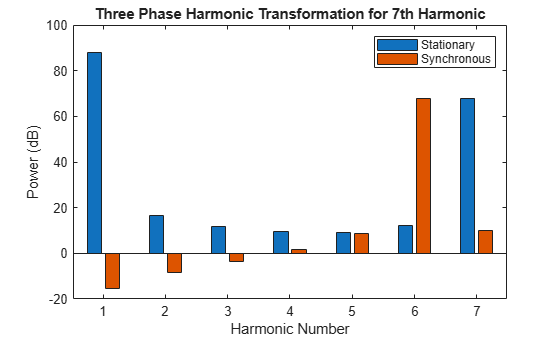
The stationary reference frame has large magnitudes for both the fundamental and the 7th harmonic, while the synchronous reference frame only has a large magnitude at the 6th harmonic. Because both the 5th and 7th harmonics shift to the 6th harmonic in the synchronous reference frame and the controllers are in this same reference frame, a single notch filter, on both D and Q axis, can be used to reduce the 6th harmonic and, therefore, the 5th and 7th harmonics in the stationary reference frame.
Using a Notch Filter to Remove the Harmonic Distortion for Variable Speeds
As discussed previously, the harmonics are multiples of the fundamental frequency of current and voltage. For a PMSM, this fundamental frequency is equal to the electrical speed of the motor. Thus, when the motor speed changes so does the fundamental frequency and the associated harmonics. For a motor operating at different speeds this means that a notch filter tuned at a single frequency is not sufficient. In addition, with a PMSM, a higher speed can require a higher amplitude of current and voltage which results in higher values for the harmonics as well. Because of this, it is desirable to have a notch filter that not only changes its frequency placement in real-time but also its depth as well.
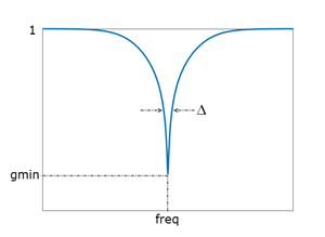
As motor speed increases, the spacing between harmonics also increases which also allows the use of a notch filter with greater width. The wider the notch filter, the larger the frequency band it affects. But this also means that the frequency estimate obtained does not need to be as accurate. In this example, you estimate the frequency of the notch filter through the use of FFTs and use an extremum seeking algorithm to adjust the notch depth and width in order to filter out the 5th and 7th harmonics regardless of the motor speed. There are several blocks and algorithms needed to construct an adaptive notch filter.
Adaptive Notch Filter (ANF) Overview
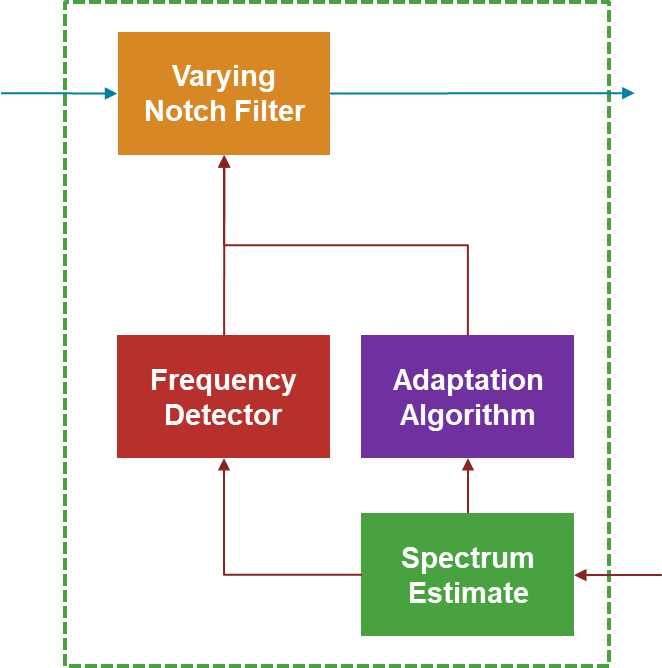
The preceding figure shows a block diagram for the adaptive notch filter (ANF) used in this example. The ANF consists of four main parts:
Adaptation Algorithm
Spectrum Estimate
Frequency Detector
Notch Filter
For this example, the Adaptation Algorithm, Frequency Detector and Notch Filter are all contained within the Adaptive Notch Filter block while the Spectrum Estimate uses the Spectrum Estimator block from DSP System Toolbox™ library. The following sections discuss the details of these blocks and functions.
Spectrum Estimation
The Adaptive Notch Filter block requires an estimate of the power spectrum to estimate the frequency placement of the notch and tune its width and depth. The power spectrum of the synchronous frame currents for D and Q is required. To obtain the spectrum, you can use the Spectrum Estimator block. The spectrum estimate is set to use 2048 frequency bands and obtain the one-sided spectrum.
Using PI Control to Reduce the Harmonic Distortion
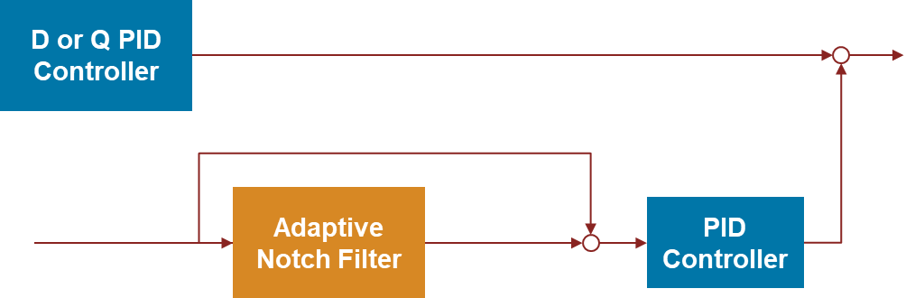
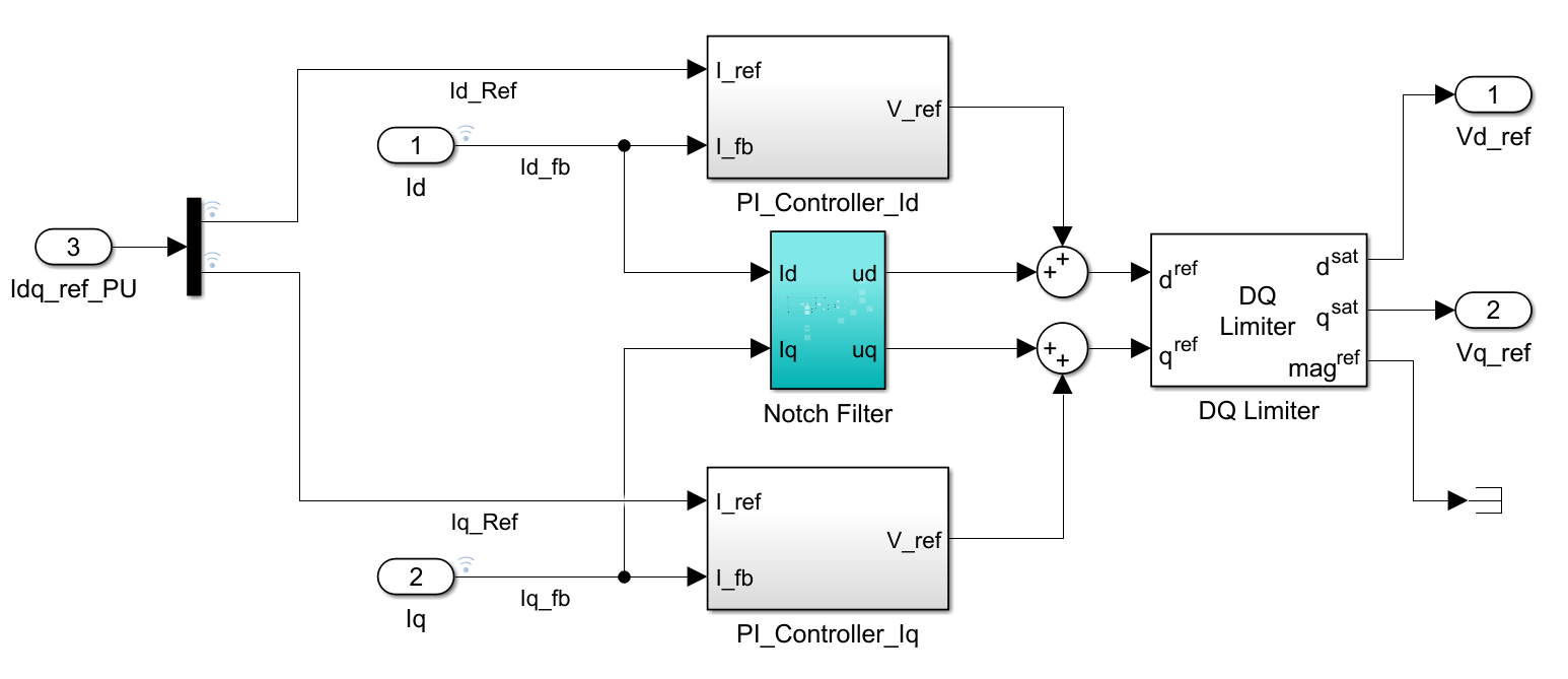
The harmonic distortion present in the motor currents is created through dead-time. In other notch filter applications, the notch filter is added in series with the upstream PID controller. Because it is desired to cancel the 6th harmonic, frequency content that has the same phase, frequency and amplitude as the 6th harmonic needs to be injected. To achieve this the D and Q axis currents can be filtered using the ANF to remove the 6th harmonic and then subtract the signal before and after the notch to obtain currents that contain only the 6th harmonic. The value of this signal represents the 6th harmonic to reduce to zero so this can be used this as the error signal input to a PI controller. The output of this PI controller will be added to the voltage reference of the current control loops as a feed forward injection. The block diagram for this process is shown below.
Using ANF to Reduce 5th and 7th Harmonic Distortion for Variable Speeds
As discussed in the previous sections, the ANF along with a PI controller can be used to obtain a feed forward voltage injection to reduce the 6th harmonic in the synchronous frame for both the D and Q axis currents. The 6th harmonic, when transformed to the stationary reference frame, becomes the 5th and 7th harmonic which are present due to the dead-time distortion.
In this example separate ANFs are applied to the D and Q axis currents as shown below.
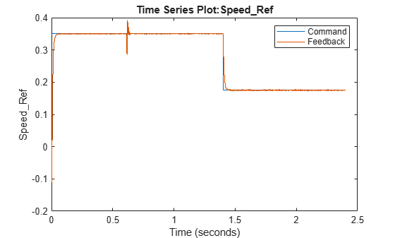
The system is first commanded to 0.35 per unit speed and then, at 1.4 seconds, commanded to 0.175 per unit speed. During the entire simulation the ANF is enabled and will become active once an estimate of the frequency location is obtained. The goal of the ANF is to reduce the magnitudes of the 5th and 7th harmonics (in the stationary reference frame) and the total harmonic distortion.
% Simulating the model takes a long time so data from a Simulation run is provided for convenience
% Model can be run using the below command if desired
sim(mdl)
% Load Saved Data
load("DataMotorANF.mat")

% Plot of Speed Command and Feedback
figure
plot(logsout{7}.Values)
hold on
plot(logsout{6}.Values)
hold off
legend("Command","Feedback")
Total Harmonic Distortion Reduced
Plot the time-domain plot of the stationary frame phase A and B currents.
% Plot of phase currents
figure
plot(0:Ts:2.4,Iab_PU)
xlabel("Time (sec)")
ylabel("Iab PU")
title("Phase A and B Currents")
xlim([1.1 1.7])
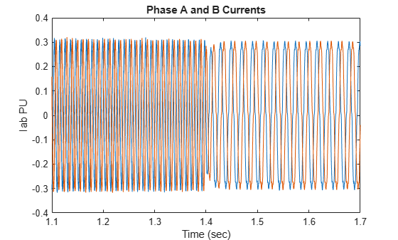
The magnitude of the phase currents remains similar at both operating speeds but the frequency of the waveform changes. This is reflected in the bar charts showing the harmonics below. In the bar graphs, you can observe that the fundamental frequency amplitude is equivalent for both speeds even though the frequency is different.
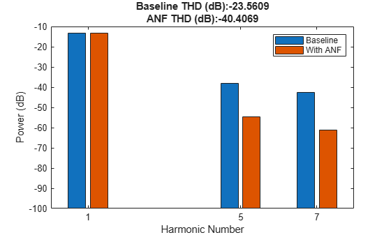
As shown in the below plots the total harmonic distortion (THD) is reduced by nearly one order of magnitude (20 dB) using the ANF and the peak values for the 5th and 7th harmonic are reduced by 18 dB and 21 dB, respectively at a motor speed of 0.35 per unit.
% Get Total Harmonic Distortion for first 9 harmonics
[r1, harmpow1, ~] = thd(Iab_PU(round(0.2/Ts):round(0.6/Ts),1),1/Ts,9);
[r2, harmpow2, ~] = thd(Iab_PU(round(1/Ts):round(1.4/Ts),1),1/Ts,9);

% Plot Harmonics before and After enabling ANF
figure
bar([1 5 7],[harmpow1([1 5 7]) harmpow2([1 5 7])],BaseValue=-100)
xlabel("Harmonic Number");ylabel("Power (dB)");legend("Baseline","With ANF")
title(["Baseline THD (dB):" + string(r1);"ANF THD (dB):" + string(r2)])
When changing speeds the ANF adapts to the new operating speed and results in similar performance across the speed range. The below figures show the total harmonic distortion after the motor has changed its speed from 0.35 per unit to 0.175 per unit.
% Get Total Harmonic Distortion for first 9 harmonics
[r3, harmpow3, ~] = thd(Iab_PU(round(1.5/Ts):round(1.8/Ts),1),1/Ts,9);
[r4, harmpow4, ~] = thd(Iab_PU(round(1.9/Ts):round(2.4/Ts),1),1/Ts,9);

% Plot Harmonics before and After enabling ANF
figure
bar([1 5 7],[harmpow1([1 5 7]) harmpow2([1 5 7]) harmpow3([1 5 7]) harmpow4([1 5 7])],BaseValue=-100)
xlabel("Harmonic Number");ylabel("Power (dB)");legend("Baseline 0.35","With ANF 0.35","Baseline 0.175","With ANF 0.175")
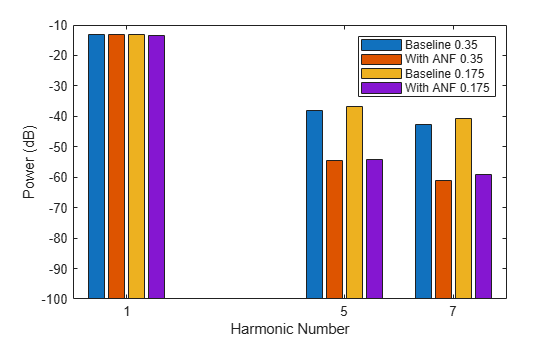
As shown in the above plots the THD remains low after the ANF has adapted to the new operating frequency. Using the ANF allows for a single notch filter to be used across the entire speed range instead of requiring multiple static notch filters.
Summary
As shown in this example, the 5th and 7th harmonic distortion caused by dead-time distortion in a PMSM is reduced using the Adaptive Notch Filter block in Simulink® Control Design™. The adaptive notch filter is applied to both D and Q axis current control loops on the 6th harmonic and both the 5th and 7th harmonics as well as the total harmonic distortion are reduced.