Design Optimization to Meet Step Response Requirements (Code)
This example shows how to programmatically optimize controller parameters to meet step response requirements using the sdo.optimize function.
Model Structure
This example uses the watertank_stepinput model. This model includes the nonlinear Water-Tank System plant and a PI controller in a single-loop feedback system.
Open the model.
sys = 'watertank_stepinput';
open_system(sys)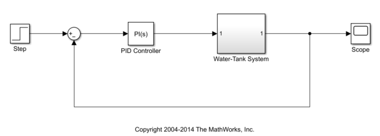
To view the water tank model, open the Water-Tank System subsystem.
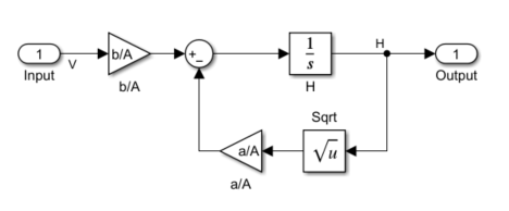
This model represents the following water tank system.
Here:
is the volume of water in the tank.
is the cross-sectional area of the tank.
is the height of water in the tank.
is the voltage applied to the pump.
is a constant related to the flow rate into the tank.
is a constant related to the flow rate out of the tank.
Water enters the tank at the top at a rate proportional to the valve opening. The valve opening is proportional to the voltage, , applied to the pump. The water leaves through an opening in the tank base at a rate that is proportional to the square root of the water height, . The presence of the square root in the water flow rate results in a nonlinear plant. Based on these flow rates, the rate of change of the tank volume is:
.
Design Requirements
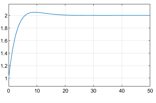
The height of water in the tank, H, must meet the following step response requirements:
Rise time less than 2.5 seconds
Settling time less than 20 seconds
Overshoot less than 5%
Specify Step Response Requirements
During optimization, the model is simulated using the current value of the model parameters and the logged signal is used to evaluate the design requirements.
For this model, log the water level, H.
PlantOutput = Simulink.SimulationData.SignalLoggingInfo;
PlantOutput.BlockPath               = [sys '/Water-Tank System'];
PlantOutput.OutputPortIndex         = 1;
PlantOutput.LoggingInfo.NameMode    = 1;
PlantOutput.LoggingInfo.LoggingName = 'PlantOutput';
Next, create a sdo.SimulationTest object to store the logging information. You also use this later to simulate the model.
simulator = sdo.SimulationTest(sys);
simulator.LoggingInfo.Signals = PlantOutput;
Specify the step response requirements.
StepResp = sdo.requirements.StepResponseEnvelope;
StepResp.RiseTime = 2.5;
StepResp.SettlingTime = 20;
StepResp.PercentOvershoot = 5;
StepResp.FinalValue = 2;
StepResp.InitialValue = 1;
StepResp is a sdo.requirements.StepResponseEnvelope object. The values assigned to StepResp.FinalValue and StepResp.InitialValue correspond to a step change in the water tank height from 1 to 2.
Specify Design Variables
When you optimize the model response, the software modifies parameter (design variable) values to meet the design requirements.
Select model parameters to optimize. Here, optimize the parameters of the PID controller.
p = sdo.getParameterFromModel(sys,{'Kp','Ki'});p is an array of two param.Continuous objects.
To limit the parameters to positive values, set the minimum value of each parameter to 0.
p(1).Minimum = 0;
p(2).Minimum = 0;
Optimize Model Response
Create a design function to evaluate the system performance for a set of parameter values.
evalDesign = @(p) sldo_model1_design(p,simulator,StepResp);
evalDesign is an anonymous function that calls the cost function sldo_model1_design. The cost function simulates the model and evaluates the design requirements. To view this function, type edit sldo_model1_design at command line.
Compute the initial model response using the current values of the design variables.
initDesign = evalDesign(p);
Examine the nonlinear inequality constraints.
initDesign.Cleq
ans = 8×1

    0.1739
    0.0169
   -0.0002
   -0.0101
   -0.0229
    0.0073
   -0.0031
    0.0423
Some Cleq values are positive, beyond the specified tolerance, which indicates the response using the current parameter values violate the design requirements.
Specify optimization options.
opt = sdo.OptimizeOptions;
opt.MethodOptions.Algorithm = 'sqp';
The software configures opt to use the default optimization method, fmincon, and the sequential quadratic programming algorithm for fmincon.
Optimize the response.
[pOpt,optInfo] = sdo.optimize(evalDesign,p,opt);
 Optimization started 2026-Apr-19, 06:55:59

                               max                     First-order
 Iter F-count        f(x)   constraint    Step-size    optimality
    0      5            0       0.1739
    1     10            0      0.03411            1         0.81
    2     15            0            0        0.235       0.0429
    3     15            0            0     5.76e-19            0
Local minimum found that satisfies the constraints.

Optimization completed because the objective function is non-decreasing in
feasible directions, to within the value of the optimality tolerance,
and constraints are satisfied to within the value of the constraint tolerance.
At each optimization iteration, the software simulates the model and the default optimization solver fmincon modifies the design variables to meet the design requirements. For more information, see How the Optimization Algorithm Formulates Minimization Problems.
The message Local minimum found that satisfies the constraints indicates that the optimization solver found a solution that meets the design requirements within specified tolerances. For more information about the outputs displayed during the optimization, see Iterative Display.
Examine the optimization termination information contained in the optInfo output argument. This information helps you verify that the response meets the step response requirements.
For example, check the Cleq and exitflag fields.
Cleq shows the optimized nonlinear inequality constraints.
optInfo.Cleq
ans = 8×1

   -0.0001
   -0.0028
   -0.0050
   -0.0101
   -0.0135
   -0.0050
   -0.0050
   -0.0732
All values satisfy Cleq ≤ 0 within the optimization tolerances, which indicates that the step response requirements are satisfied.
exitflag identifies why the optimization terminated.
optInfo.exitflag
ans =
1
The value is 1, which indicates that the solver found a solution that was less than the specified tolerances on the function value and constraint violations.
View the optimized parameter values.
pOpt
pOpt(1,1) =

       Name: 'Kp'
      Value: 2.0545
    Minimum: 0
    Maximum: Inf
       Free: 1
      Scale: 1
       Info: [1×1 struct]


pOpt(2,1) =

       Name: 'Ki'
      Value: 0.3801
    Minimum: 0
    Maximum: Inf
       Free: 1
      Scale: 1
       Info: [1×1 struct]


2x1 param.Continuous
Simulate the model with the optimized values.
sdo.setValueInModel(sys,pOpt);
sim(sys);
Verify that the model output meets the step response requirements.
Close the model.
close_system(sys,0);
See Also
sdo.optimize | Simulink.SimulationData.SignalLoggingInfo | sdo.SimulationTest | sdo.getParameterFromModel | sdo.requirements.StepResponseEnvelope | param.Continuous | sdo.OptimizeOptions