Discrete-Valued Variables in Response Optimization (Code)
This example shows how to use response optimization to tune discrete-valued variables. Discrete-valued variables represent model parameters that are restricted to a finite set of values, instead of continuously varying. To use discrete-valued variables for response optimization or parameter estimation, you must use the surrogateopt solver for mixed-integer optimization.
Open the Model
In the sdoMotorPosition model, a PI controller enables the angular position of a DC motor to match a desired reference value. The load on the motor is subject to disturbances, and the controller must reject these disturbances.
open_system('sdoMotorPosition')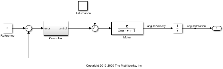
Within the Controller subsystem, the PI gains are set by a 12 V source divided down by resistors R1, R2, R3, and R4, as shown in the following diagram.
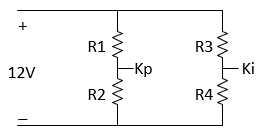
The proportional gain, Kp, is given by 12*R2/(R1+R2) and the integral gain, Ki, is given by 12*R4/(R3+R4). The initial values of the resistances are R1 = 47 kΩ, R2 = 180 kΩ, R3 = 10 kΩ, and R4 = 10 kΩ.
Specify Discrete Design Variables
Those four resistor values are the model parameters to tune for the optimization. Because resistors are only available in discrete values, use discrete parameters to represent them. To do so, use third input argument to sdo.getParameterFromModel to specify discrete parameters.
DesignVars = sdo.getParameterFromModel('sdoMotorPosition',[],{'R1','R2','R3','R4'});
sdo.getParameterFromModel returns an array of param.Discrete parameter objects that correspond to the model parameters in the order you specified. Set the ValueSet property of each parameter to the set of discrete values allowed for the parameter. Set the Value property to the current value, which must be present in ValueSet.
% R1 values
DesignVars(1).ValueSet = [39 43 47 51 56] * 1e3;
DesignVars(1).Value    = 47*1e3;
% R2 values
DesignVars(2).ValueSet = [150 160 180 200 220] * 1e3;
DesignVars(2).Value    = 180*1e3;
% R3 values
DesignVars(3).ValueSet = [8.2 9.1 10 11 12] * 1e3;
DesignVars(3).Value    = 10*1e3;
% R4 values
DesignVars(4).ValueSet = [8.2 9.1 10 11 12] * 1e3;
DesignVars(4).Value    = 10*1e3;
Specify Design Requirements and Signals
The model applies a step disturbance at 1 second. With the initial resistance values specified in the model, the disturbance causes the motor to deviate by about 20°. The response then settles back to within ±5° of the reference position by 4 seconds after the disturbance. For this example, find new resistor values to improve this specification by 10%, so that the motor deviates no more than 18°, and settles back to within ±4.5° degrees of the reference position by 4 seconds after the disturbance. First, specify these new design requirements using sdo.requirements.SignalBound.
Requirements = struct;
Requirements.UpperBound = sdo.requirements.SignalBound(...
    'BoundMagnitudes', [18 18 ; 4.5 4.5], ...
    'BoundTimes', [1 5 ; 5 15]);
Requirements.LowerBound = sdo.requirements.SignalBound(...
    'BoundMagnitudes', [-4.5 -4.5], ...
    'BoundTimes', [5 15], ...
    'Type', '>=');
To visualize the initial performance against the requirement, first specify signals to log during simulation. In particular, log the output of the Integrator block, which is the angular position of the model, the signal you want to optimize. To do so, create a simulation scenario with sdo.SimulationTest and configure its LoggingInfo property. Also, to prepare the scenario for later use in the optimization, assign the design variables you created as its Parameters property.
Simulator = sdo.SimulationTest('sdoMotorPosition');

Sig_Info = Simulink.SimulationData.SignalLoggingInfo;
Sig_Info.BlockPath = 'sdoMotorPosition/Integrator';
Sig_Info.LoggingInfo.LoggingName = 'Sig';
Sig_Info.LoggingInfo.NameMode = 1;

Simulator.LoggingInfo.Signals = Sig_Info;

Simulator.Parameters = DesignVars;
Now create a plot of the disturbance-rejection requirements. Then, simulate the model and add the logged signal to the plot.
hRequirement = plot( ...
    Requirements.LowerBound.BoundTimes', ...
    Requirements.LowerBound.BoundMagnitudes', ...
    'color','black');
hold on
plot( ...
    Requirements.UpperBound.BoundTimes', ...
    Requirements.UpperBound.BoundMagnitudes', ...
    'color','black');
% Simulator.Parameters = DesignVars;
Simulator = sim(Simulator);
SimLog = find(Simulator.LoggedData, ...
    get_param('sdoMotorPosition','SignalLoggingName'));
Sig_Log = find(SimLog,'Sig');
clrs = colororder;
hOriginal = plot(Sig_Log.Values,'Color',clrs(2,:));
legend([hRequirement hOriginal],'Requirement','Original Variables');
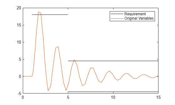
The plot shows that the current resistor values do not quite satisfy the more stringent requirement.
Set Up Optimization
The optimization process runs the model many times with different values for the resistor variables. To expedite this, configure the simulator for fast restart.
Simulator = setup(Simulator,FastRestart='on');Optimization requires an objective or cost function that runs the model and determines whether the disturbance rejection requirements are satisfied. For this example, use the function sdoMotorPosition_optFcn, which is included at the end of the example. This function is called many times by the optimization solver. To pass the function to the optimizer, use an anonymous function with one argument that calls sdoMotorPosition_optFcn.
optimfcn = @(P) sdoMotorPosition_optFcn(P,Simulator,Requirements);
Specify optimization options. Set the optimization method to surrogateopt solver, which is the method that supports tuning of discrete parameters.
Options = sdo.OptimizeOptions;
Options.Method = 'surrogateopt';
Options.MethodOptions.MaxFunctionEvaluations = 100;
Options.MethodOptions.ObjectiveLimit = 0.001;
Options.OptimizedModel = Simulator;
Optimize the Design
To find resistance values optimized for the requirements, call sdo.optimize with the cost function handle, parameters to optimize, and options.
rng('default');   % for reproducibility
[Optimized_DesignVars,Info] = sdo.optimize(optimfcn,DesignVars,Options);
 Optimization started 2026-Apr-19, 07:05:21

                                       Current
 F-count     max constraint     max constraint     Trial type
       1          0.0759805          0.0759805     initial
       2          0.0751287          0.0751287     random
       3          0.0751287           0.179179     random
       4          0.0447169          0.0447169     random
       5          0.0317818          0.0317818     random
       6          0.0317818           0.261353     random
       7          0.0257711          0.0257711     random
       8          0.0257711          0.0930365     random
       9          0.0257711          0.0971938     random
      10          0.0257711           0.200359     random
      11          0.0062997          0.0062997     random
      12          0.0062997           0.206374     random
      13          0.0062997          0.0818387     random
      14          0.0062997          0.0585416     random
      15          0.0062997           0.114002     random
      16          0.0062997           0.112485     random
      17          0.0062997          0.0759805     random
      18          0.0062997          0.0709489     random
      19          0.0062997           0.280136     random
      20          0.0062997           0.099985     random
      21                  0                  0     adaptive
      22                  0          0.0691728     random
      23                  0          0.0347164     random
      24                  0          0.0977682     random
      25                  0          0.0589627     random
      26                  0           0.131778     random
      27                  0           0.147347     random
      28                  0           0.104488     random
      29                  0          0.0534262     random
      30                  0             0.1643     random
      31                  0          0.0419731     random
      32                  0          0.0396579     random
      33                  0           0.077945     random
      34                  0          0.0883493     random
      35                  0                  0     random
      36                  0          0.0455853     random
      37                  0            0.13976     random
      38                  0           0.140634     random
      39                  0          0.0662368     random
      40                  0           0.256738     random
      41                  0          0.0348764     random
      42                  0            0.18995     random
      43                  0          0.0615952     random
      44                  0          0.0597358     random
      45                  0           0.015983     random
      46                  0          0.0770592     random
      47                  0           0.174666     random
      48                  0           0.081758     random
      49                  0          0.0240828     random
      50                  0           0.173292     random

                                       Current
 F-count     max constraint     max constraint     Trial type
      51                  0           0.116519     random
      52                  0           0.217099     random
      53                  0           0.104371     random
      54                  0          0.0937562     random
      55                  0           0.104225     random
      56                  0          0.0380129     random
      57                  0           0.150819     random
      58                  0          0.0636666     random
      59                  0          0.0320499     random
      60                  0          0.0273158     random
      61                  0          0.0798937     random
      62                  0           0.174146     random
      63                  0          0.0166127     random
      64                  0         0.00433873     adaptive
      65                  0           0.294106     random
      66                  0                  0     adaptive
      67                  0          0.0319864     random
      68                  0           0.266843     random
      69                  0          0.0342618     random
      70                  0          0.0982987     random
      71                  0          0.0419731     random
      72                  0          0.0396579     random
      73                  0           0.299815     random
      74                  0          0.0712971     random
      75                  0          0.0709489     random
      76                  0          0.0589627     random
      77                  0           0.131778     random
      78                  0         0.00653156     random
      79                  0           0.211877     random
      80                  0          0.0967155     random
      81                  0          0.0689487     random
      82                  0          0.0257711     random
      83                  0          0.0930365     random
      84                  0           0.114002     random
      85                  0           0.112485     random
      86                  0            0.06706     random
      87                  0          0.0751287     random
      88                  0                  0     adaptive
      89                  0          0.0759805     random
      90                  0            0.10447     random
      91                  0           0.190644     random
      92                  0           0.142755     random
      93                  0           0.104193     random
      94                  0           0.100237     random
      95                  0           0.097787     random
      96                  0          0.0735855     random
      97                  0           0.137557     random
      98                  0          0.0783709     random
      99                  0          0.0875674     random
     100                  0          0.0794652     random
     101                  0                  0     best value
The current solution is feasible. surrogateopt stopped because it exceeded the function evaluation limit set by the 'MethodOptions.MaxFunctionEvaluations' property in the sdo.OptimizeOptions object.
If the solution needs to be improved, you could try increasing the function evaluation limit.
Evaluate Optimized Design
Plot the model response after optimization.
Simulator.Parameters = Optimized_DesignVars;
Simulator = sim(Simulator);
SimLog = find(Simulator.LoggedData, ...
    get_param('sdoMotorPosition','SignalLoggingName'));
Sig_Log = find(SimLog,'Sig');
clrs = colororder;
hOptimized = plot(Sig_Log.Values, 'Color', clrs(1,:));
legend([hRequirement hOriginal hOptimized], ...
    'Requirement','Original Variables','Optimized Variables');
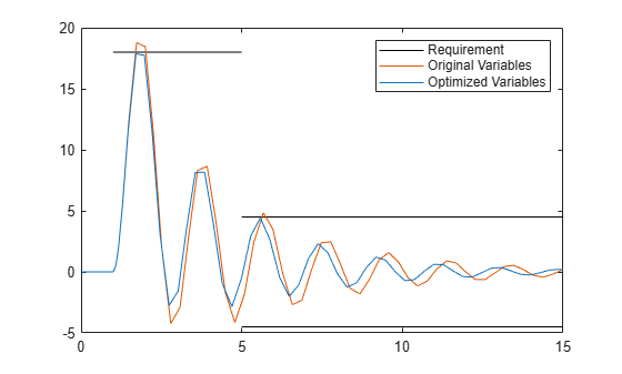
Now the motor position is within the spec of the disturbance rejection requirement.
Update Model with Optimized Parameter Values
sdo.Optimize returns tuned versions of the parameters in the array Optimized_DesignVars. Each entry in this array is a param.Discrete parameter object whose Value property is set to the optimized value. For instance, examine the new value of R2.
Optimized_DesignVars(2).Value
ans =
220000
Update the model with the optimized parameter values.
sdo.setValueInModel('sdoMotorPosition',Optimized_DesignVars);Restore the simulator fast restart settings.
Simulator = restore(Simulator);
Conclusion
In this example you tuned variables to improve the disturbance rejection characteristics of a motor controller. The variables being tuned were electrical component parts that could only take on discrete values, rather than continuous values. You used sdo.getParameterFromModel to specify the variables as discrete, and used the surrogateopt solver to tune the parameters.
Objective Function
The function sdoMotorPosition_optFcn is called at each iteration of the optimization problem with a set of parameter values, P. The function returns the objective value and constraint violations, Vals, to the optimization solver. See sdo.optimize for a more detailed description of the function signature.
function Vals = sdoMotorPosition_optFcn(P,Simulator,Requirements)
%SDOMOTORPOSITION_OPTFCN
%

% Simulate the model.
Simulator.Parameters = P;
Simulator = sim(Simulator);

% Retrieve logged signal data.
SimLog = find(Simulator.LoggedData, ...
    get_param('sdoMotorPosition','SignalLoggingName'));
Sig_Log = find(SimLog,'Sig');

% Evaluate the design requirements.
Cleq_UpperBound = evalRequirement( ...
    Requirements.UpperBound,Sig_Log.Values);
Cleq_LowerBound = evalRequirement( ...
    Requirements.LowerBound,Sig_Log.Values);

% Collect the evaluated design requirement values in a structure to
% return to the optimization solver.
Vals.Cleq = [...
    Cleq_UpperBound(:); ...
    Cleq_LowerBound(:)];
end
See Also
sdo.optimize | param.Discrete | sdo.getParameterFromModel | sdo.OptimizeOptions