Examine the Gaussian Mixture Assumption
Discriminant analysis assumes that the data comes from a Gaussian mixture model (see Creating Discriminant Analysis Model). If the data appears to come from a Gaussian mixture model, you can expect discriminant analysis to be a good classifier. Furthermore, the default linear discriminant analysis assumes that all class covariance matrices are equal. This section shows methods to check these assumptions:
Bartlett Test of Equal Covariance Matrices for Linear Discriminant Analysis
The Bartlett test (see Box [1]) checks equality of the covariance matrices of the various classes. If the covariance matrices are equal, the test indicates that linear discriminant analysis is appropriate. If not, consider using quadratic discriminant analysis, setting the DiscrimType name-value pair argument to 'quadratic' in fitcdiscr.
The Bartlett test assumes normal (Gaussian) samples, where neither the means nor covariance matrices are known. To determine whether the covariances are equal, compute the following quantities:
Sample covariance matrices per class Σi, 1 ≤ i ≤ k, where k is the number of classes.
Pooled-in covariance matrix Σ.
Test statistic V:
where n is the total number of observations, ni is the number of observations in class i, and |Σ| means the determinant of the matrix Σ.
Asymptotically, as the number of observations in each class ni becomes large, V is distributed approximately χ2 with kd(d + 1)/2 degrees of freedom, where d is the number of predictors (number of dimensions in the data).
The Bartlett test is to check whether V exceeds a given percentile of the χ2 distribution with kd(d + 1)/2 degrees of freedom. If it does, then reject the hypothesis that the covariances are equal.
Bartlett Test of Equal Covariance Matrices
Check whether the Fisher iris data is well modeled by a single Gaussian covariance, or whether it is better modeled as a Gaussian mixture by performing a Bartlett test of equal covariance matrices.
Load the fisheriris data set.
load fisheriris;
prednames = {'SepalLength','SepalWidth','PetalLength','PetalWidth'};
When all the class covariance matrices are equal, a linear discriminant analysis is appropriate.
Train a linear discriminant analysis model (the default type) using the Fisher iris data.
L = fitcdiscr(meas,species,'PredictorNames',prednames);When the class covariance matrices are not equal, a quadratic discriminant analysis is appropriate.
Train a quadratic discriminant analysis model using the Fisher iris data and compute statistics
Q = fitcdiscr(meas,species,'PredictorNames',prednames,'DiscrimType','quadratic');
Store as variables the number of observations N, dimension of the data set D, number of classes K, and number of observations in each class Nclass.
[N,D] = size(meas)
N =
150
D =
4
K = numel(unique(species))
K =
3
Nclass = grpstats(meas(:,1),species,'numel')'Nclass = 1×3
50 50 50
Compute the test statistic V.
SigmaL = L.Sigma;
SigmaQ = Q.Sigma;
V = (N-K)*log(det(SigmaL));
for k=1:K
    V = V - (Nclass(k)-1)*log(det(SigmaQ(:,:,k)));
end
V
V =
146.6632
Compute the p-value.
nu = K*D*(D+1)/2;
pval1 = chi2cdf(V,nu,'upper')
pval1 = 2.6091e-17
Because pval1 is smaller than 0.05, the Bartlett test rejects the hypothesis of equal covariance matrices. The result indicates to use quadratic discriminant analysis, as opposed to linear discriminant analysis.
Q-Q Plot
A Q-Q plot graphically shows whether an empirical distribution is close to a theoretical distribution. If the two are equal, the Q-Q plot lies on a 45° line. If not, the Q-Q plot strays from the 45° line.
Compare Q-Q Plots for Linear and Quadratic Discriminants
Analyze the Q-Q plots to check whether the Fisher iris data is better modeled by a single Gaussian covariance or as a Gaussian mixture.
Load the fisheriris data set.
load fisheriris;
prednames = {'SepalLength','SepalWidth','PetalLength','PetalWidth'};
When all the class covariance matrices are equal, a linear discriminant analysis is appropriate.
Train a linear discriminant analysis model.
L = fitcdiscr(meas,species,'PredictorNames',prednames);When the class covariance matrices are not equal, a quadratic discriminant analysis is appropriate.
Train a quadratic discriminant analysis model using the Fisher iris data.
Q = fitcdiscr(meas,species,'PredictorNames',prednames,'DiscrimType','quadratic');
Compute the number of observations, dimension of the data set, and expected quantiles.
[N,D] = size(meas);
expQuant = chi2inv(((1:N)-0.5)/N,D);
Compute the observed quantiles for the linear discriminant model.
obsL = mahal(L,L.X,'ClassLabels',L.Y);
[obsL,sortedL] = sort(obsL);
Graph the Q-Q plot for the linear discriminant.
figure;
gscatter(expQuant,obsL,L.Y(sortedL),'bgr',[],[],'off');
legend('virginica','versicolor','setosa','Location','NW');
xlabel('Expected quantile');
ylabel('Observed quantile for LDA');
line([0 20],[0 20],'color','k');
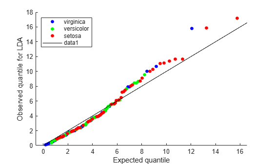
The expected and observed quantiles agree somewhat. The deviation of the plot from the 45° line upward indicates that the data has heavier tails than a normal distribution. The plot shows three possible outliers at the top: two observations from class 'setosa' and one observation from class 'virginica'.
Compute the observed quantiles for the quadratic discriminant model.
obsQ = mahal(Q,Q.X,'ClassLabels',Q.Y);
[obsQ,sortedQ] = sort(obsQ);
Graph the Q-Q plot for the quadratic discriminant.
figure;
gscatter(expQuant,obsQ,Q.Y(sortedQ),'bgr',[],[],'off');
legend('virginica','versicolor','setosa','Location','NW');
xlabel('Expected quantile');
ylabel('Observed quantile for QDA');
line([0 20],[0 20],'color','k');
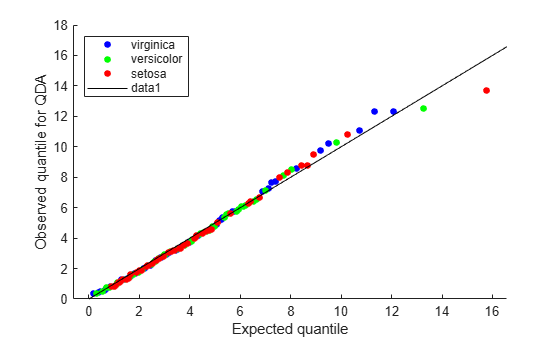
The Q-Q plot for the quadratic discriminant shows a better agreement between the observed and expected quantiles. The plot shows only one possible outlier from class 'setosa'. The Fisher iris data is better modeled as a Gaussian mixture with covariance matrices that are not required to be equal across classes.
Mardia Kurtosis Test of Multivariate Normality
The Mardia kurtosis test (see Mardia [2]) is an alternative to examining a Q-Q plot. It gives a numeric approach to deciding if data matches a Gaussian mixture model.
In the Mardia kurtosis test you compute M, the mean of the fourth power of the Mahalanobis distance of the data from the class means. If the data is normally distributed with a constant covariance matrix (and is thus suitable for linear discriminant analysis), M is asymptotically distributed as normal with mean d(d + 2) and variance 8d(d + 2)/n, where
d is the number of predictors (number of dimensions in the data).
n is the total number of observations.
The Mardia test is two sided: check whether M is close enough to d(d + 2) with respect to a normal distribution of variance 8d(d + 2)/n.
Mardia Kurtosis Test for Linear and Quadratic Discriminants
Perform a Mardia kurtosis tests to check whether the Fisher iris data is approximately normally distributed for both linear and quadratic discriminant analyses.
Load the fisheriris data set.
load fisheriris;
prednames = {'SepalLength','SepalWidth','PetalLength','PetalWidth'};
When all the class covariance matrices are equal, a linear discriminant analysis is appropriate.
Train a linear discriminant analysis model.
L = fitcdiscr(meas,species,'PredictorNames',prednames);When the class covariance matrices are not equal, a quadratic discriminant analysis is appropriate.
Train a quadratic discriminant analysis model using the Fisher iris data.
Q = fitcdiscr(meas,species,'PredictorNames',prednames,'DiscrimType','quadratic');
Compute the mean and variance of the asymptotic distribution.
[N,D] = size(meas);
meanKurt = D*(D+2)
meanKurt =
24
varKurt = 8*D*(D+2)/N
varKurt =
1.2800
Compute the p-value for the Mardia kurtosis test on the linear discriminant model.
mahL = mahal(L,L.X,'ClassLabels',L.Y);
meanL = mean(mahL.^2);
[~,pvalL] = ztest(meanL,meanKurt,sqrt(varKurt))
pvalL = 0.0208
Because pvalL is smaller than 0.05, the Mardia kurtosis test rejects the hypothesis of the data being normally distributed with a constant covariance matrix.
Compute the p-value for the Mardia kurtosis test on the quadratic discriminant model.
mahQ = mahal(Q,Q.X,'ClassLabels',Q.Y);
meanQ = mean(mahQ.^2);
[~,pvalQ] = ztest(meanQ,meanKurt,sqrt(varKurt))
pvalQ = 0.7230
Because pvalQ is greater than 0.05, the data is consistent with the multivariate normal distribution.
The results indicate to use quadratic discriminant analysis, as opposed to linear discriminant analysis.
References
[1] Box, G. E. P. “A General Distribution Theory for a Class of Likelihood Criteria.” Biometrika 36, no. 3–4 (1949): 317–46. https://doi.org/10.1093/biomet/36.3-4.317.
[2] Mardia, K. V. “Measures of Multivariate Skewness and Kurtosis with Applications.” Biometrika 57, no. 3 (1970): 519–30. https://doi.org/10.1093/biomet/57.3.519.