Main Content

friedman

Friedman’s test

Description

example

p = friedman(x,reps) returns the p-value for the nonparametric Friedman's test to compare column effects in a two-way layout. friedman tests the null hypothesis that the column effects are all the same against the alternative that they are not all the same. Friedman's test provides an analysis that is similar to a two-way ANOVA without interactions. For more information, see Friedman’s Test.

p = friedman(x,reps,displayopt) enables the ANOVA table display when displayopt is 'on' (default) and suppresses the display when displayopt is 'off'.

[p,tbl] = friedman(___) returns the ANOVA table (including column and row labels) in cell array tbl.

[p,tbl,stats] = friedman(___) also returns a structure stats that you can use to perform a follow-up multiple comparison test.

Examples

collapse all

This example shows how to test for column effects in a two-way layout using Friedman's test.

Load the sample data.

load popcorn
popcorn
popcorn = 6×3

    5.5000    4.5000    3.5000
    5.5000    4.5000    4.0000
    6.0000    4.0000    3.0000
    6.5000    5.0000    4.0000
    7.0000    5.5000    5.0000
    7.0000    5.0000    4.5000

This data comes from a study of popcorn brands and popper type (Hogg 1987). The columns of the matrix popcorn are brands (Gourmet, National, and Generic). The rows are popper type (Oil and Air). The study popped a batch of each brand three times with each popper. The values are the yield in cups of popped popcorn.

Use Friedman's test to determine whether the popcorn brand affects the yield of popcorn.

p = friedman(popcorn,3)
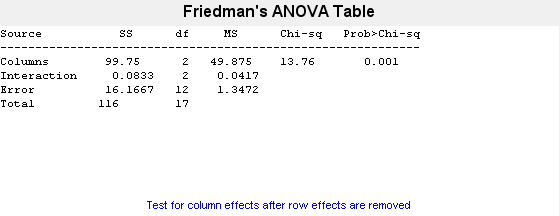
Figure Friedman's Test contains objects of type uicontrol.

p = 0.0010

The small value of p = 0.001 indicates the popcorn brand affects the yield of popcorn.

Input Arguments

collapse all

Sample data for the hypothesis test, specified as a matrix. The columns of x represent changes in a factor A. The rows represent changes in a blocking factor B. If there is more than one observation for each combination of factors, input reps indicates the number of replicates in each “cell,” which must be constant.

Data Types: single | double

Number of replicates for each combination of groups, specified as a positive integer value. For example, the following data has two replicates (reps = 2) for each group combination of row factor A and column factor B.

B=1B=2[x111x121x112x122x211x221x212x222x311x321x312x322]}A=1}A=2}A=3

Data Types: single | double

ANOVA table display option, specified as 'off' or 'on'.

If displayopt is 'on', then friedman displays a figure showing an ANOVA table, which divides the variability of the ranks into two or three parts:

  • The variability due to the differences among the column effects

  • The variability due to the interaction between rows and columns (if reps is greater than its default value of 1)

  • The remaining variability not explained by any systematic source

The ANOVA table has six columns:

  • The first shows the source of the variability.

  • The second shows the Sum of Squares (SS) due to each source.

  • The third shows the degrees of freedom (df) associated with each source.

  • The fourth shows the Mean Squares (MS), which is the ratio SS/df.

  • The fifth shows Friedman's chi-square statistic.

  • The sixth shows the p value for the chi-square statistic.

You can copy a text version of the ANOVA table to the clipboard by selecting Copy Text from the Edit menu.

Output Arguments

collapse all

p-value of the test, returned as a scalar value in the range [0,1]. p is the probability of observing a test statistic as extreme as, or more extreme than, the observed value under the null hypothesis. Small values of p cast doubt on the validity of the null hypothesis.

ANOVA table, including column and row labels, returned as a cell array. The ANOVA table has six columns:

  • The first shows the source of the variability.

  • The second shows the Sum of Squares (SS) due to each source.

  • The third shows the degrees of freedom (df) associated with each source.

  • The fourth shows the Mean Squares (MS), which is the ratio SS/df.

  • The fifth shows Friedman's chi-square statistic.

  • The sixth shows the p value for the chi-square statistic.

You can copy a text version of the ANOVA table to the clipboard by selecting Copy Text from the Edit menu.

Test data, returned as a structure. friedman evaluates the hypothesis that the column effects are all the same against the alternative that they are not all the same. However, sometimes it is preferable to perform a test to determine which pairs of column effects are significantly different, and which are not. You can use the multcompare function to perform such tests by supplying stats as the input value.

More About

collapse all

Friedman’s Test

Friedman's test is similar to classical balanced two-way ANOVA, but it tests only for column effects after adjusting for possible row effects. It does not test for row effects or interaction effects. Friedman's test is appropriate when columns represent treatments that are under study, and rows represent nuisance effects (blocks) that need to be taken into account but are not of any interest.

The different columns of X represent changes in a factor A. The different rows represent changes in a blocking factor B. If there is more than one observation for each combination of factors, input reps indicates the number of replicates in each “cell,” which must be constant.

The matrix below illustrates the format for a set-up where column factor A has three levels, row factor B has two levels, and there are two replicates (reps=2). The subscripts indicate row, column, and replicate, respectively.

[x111x121x131x112x122x132x211x221x231x212x222x232]

Friedman's test assumes a model of the form

xijk=μ+αi+βj+εijk

where μ is an overall location parameter, αi represents the column effect,βj represents the row effect, and εijk represents the error. This test ranks the data within each level of B, and tests for a difference across levels of A. The p that friedman returns is the p value for the null hypothesis that αi=0. If the p value is near zero, this casts doubt on the null hypothesis. A sufficiently small p value suggests that at least one column-sample median is significantly different than the others; i.e., there is a main effect due to factor A. The choice of a critical p value to determine whether a result is “statistically significant” is left to the researcher. It is common to declare a result significant if the p value is less than 0.05 or 0.01.

Friedman's test makes the following assumptions about the data in X:

  • All data come from populations having the same continuous distribution, apart from possibly different locations due to column and row effects.

  • All observations are mutually independent.

The classical two-way ANOVA replaces the first assumption with the stronger assumption that data come from normal distributions.

References

[1] Hogg, R. V., and J. Ledolter. Engineering Statistics. New York: MacMillan, 1987.

[2] Hollander, M., and D. A. Wolfe. Nonparametric Statistical Methods. Hoboken, NJ: John Wiley & Sons, Inc., 1999.

Version History

Introduced before R2006a