kruskalwallis
Kruskal-Wallis test
Syntax
Description
p = kruskalwallis(x)x comes from the same distribution, using the
Kruskal-Wallis test. The
alternative hypothesis is that not all samples come from the same distribution. The
Kruskal-Wallis test provides a nonparametric alternative to a one-way ANOVA. For
more information, see Kruskal-Wallis Test.
p = kruskalwallis(x,group,displayopt)
Examples
Create two different normal probability distribution objects. The first distribution has mu = 0 and sigma = 1, and the second distribution has mu = 2 and sigma = 1.
pd1 = makedist('Normal');
pd2 = makedist('Normal','mu',2,'sigma',1);
Create a matrix of sample data by generating random numbers from these two distributions.
rng('default'); % for reproducibility
x = [random(pd1,20,2),random(pd2,20,1)];
The first two columns of x contain data generated from the first distribution, while the third column contains data generated from the second distribution.
Test the null hypothesis that the sample data from each column in x comes from the same distribution.
p = kruskalwallis(x)
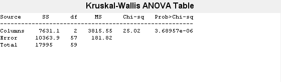

p =
3.6896e-06
The returned value of p indicates that kruskalwallis rejects the null hypothesis that all three data samples come from the same distribution at a 1% significance level. The ANOVA table provides additional test results, and the box plot visually presents the summary statistics for each column in x.
Create two different normal probability distribution objects. The first distribution has mu = 0 and sigma = 1. The second distribution has mu = 2 and sigma = 1.
pd1 = makedist('Normal');
pd2 = makedist('Normal','mu',2,'sigma',1);
Create a matrix of sample data by generating random numbers from these two distributions.
rng('default'); % for reproducibility
x = [random(pd1,20,2),random(pd2,20,1)];
The first two columns of x contain data generated from the first distribution, while the third column contains data generated from the second distribution.
Test the null hypothesis that the sample data from each column in x comes from the same distribution. Suppress the output displays, and generate the structure stats to use in further testing.
[p,tbl,stats] = kruskalwallis(x,[],'off')p = 3.6896e-06
tbl=4×6 cell array
    {'Source' }    {'SS'        }    {'df'}    {'MS'        }    {'Chi-sq'  }    {'Prob>Chi-sq'}
    {'Columns'}    {[7.6311e+03]}    {[ 2]}    {[3.8155e+03]}    {[ 25.0200]}    {[ 3.6896e-06]}
    {'Error'  }    {[1.0364e+04]}    {[57]}    {[  181.8228]}    {0×0 double}    {0×0 double   }
    {'Total'  }    {[     17995]}    {[59]}    {0×0 double  }    {0×0 double}    {0×0 double   }
stats = struct with fields:
       gnames: [3×1 char]
            n: [20 20 20]
       source: 'kruskalwallis'
    meanranks: [26.7500 18.9500 45.8000]
         sumt: 0
The returned value of p indicates that the test rejects the null hypothesis at the 1% significance level. You can use the structure stats to perform additional follow-up testing. The cell array tbl contains the same data as the graphical ANOVA table, including column and row labels.
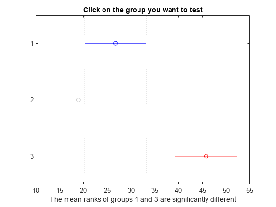
Conduct a follow-up test to identify which data sample comes from a different distribution.
c = multcompare(stats);
Note: Intervals can be used for testing but are not simultaneous confidence intervals.
Display the multiple comparison results in a table.
tbl = array2table(c,"VariableNames", ...
    ["Group A","Group B","Lower Limit","A-B","Upper Limit","P-value"])
tbl=3×6 table
    Group A    Group B    Lower Limit     A-B      Upper Limit     P-value
    _______    _______    ___________    ______    ___________    __________

       1          2         -5.1435         7.8       20.744         0.33446
       1          3         -31.994      -19.05      -6.1065       0.0016282
       2          3         -39.794      -26.85      -13.906      3.4768e-06
The results indicate that there is a significant difference between groups 1 and 3, so the test rejects the null hypothesis that the data in these two groups comes from the same distribution. The same is true for groups 2 and 3. However, there is not a significant difference between groups 1 and 2, so the test does not reject the null hypothesis that these two groups come from the same distribution. Therefore, these results suggest that the data in groups 1 and 2 come from the same distribution, and the data in group 3 comes from a different distribution.
Create a vector, strength, containing measurements of the strength of metal beams. Create a second vector, alloy, indicating the type of metal alloy from which the corresponding beam is made.
strength = [82 86 79 83 84 85 86 87 74 82 ...
            78 75 76 77 79 79 77 78 82 79];

alloy = {'st','st','st','st','st','st','st','st',...
         'al1','al1','al1','al1','al1','al1',...
         'al2','al2','al2','al2','al2','al2'};
Test the null hypothesis that the beam strength measurements have the same distribution across all three alloys.
p = kruskalwallis(strength,alloy,'off')p = 0.0018
The returned value of p indicates that the test rejects the null hypothesis at the 1% significance level.
Input Arguments
Output Arguments
More About
Version History
Introduced before R2006a