Main Content

logninv

Lognormal inverse cumulative distribution function

Description

x = logninv(p) returns the inverse of the standard lognormal cumulative distribution function (cdf), evaluated at the probability values in p. In the standard lognormal distribution, the mean and standard deviation of logarithmic values are 0 and 1, respectively.

x = logninv(p,mu) returns the inverse of the lognormal cdf with the distribution parameters mu (mean of logarithmic values) and 1 (standard deviation of logarithmic values), evaluated at the probability values in p.

example

x = logninv(p,mu,sigma) returns the inverse of the lognormal cdf with the distribution parameters mu (mean of logarithmic values) and sigma (standard deviation of logarithmic values), evaluated at the probability values in p.

[x,xLo,xUp] = logninv(p,mu,sigma,pCov) also returns the 95% confidence bounds [xLo,xUp] of x using the estimated parameters (mu and sigma) and their covariance matrix pCov.

[x,xLo,xUp] = logninv(p,mu,sigma,pCov,alpha) specifies the confidence level for the confidence interval [xLo,xUp] to be 100(1–alpha)%.

Examples

collapse all

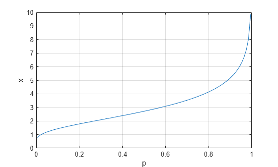
Compute the inverse of cdf values evaluated at the probability values in p for the lognormal distribution with mean mu and standard deviation sigma.

p = 0.005:0.01:0.995;
mu = 1;
sigma = 0.5;
x = logninv(p,mu,sigma);

Plot the inverse cdf.

plot(p,x)
grid on
xlabel('p');
ylabel('x');

Figure contains an axes object. The axes object with xlabel p, ylabel x contains an object of type line.

Find the maximum likelihood estimates (MLEs) of the lognormal distribution parameters, and then find the confidence interval of the corresponding inverse cdf value.

Generate 1000 random numbers from the lognormal distribution with the parameters 5 and 2.

rng('default') % For reproducibility
n = 1000; % Number of samples
x = lognrnd(5,2,[n,1]);

Find the MLEs for the distribution parameters (mean and standard deviation of logarithmic values) by using mle.

phat = mle(x,'distribution','LogNormal')
phat = 1×2

    4.9347    1.9969

muHat = phat(1);
sigmaHat = phat(2);

Estimate the covariance of the distribution parameters by using lognlike. The function lognlike returns an approximation to the asymptotic covariance matrix if you pass the MLEs and the samples used to estimate the MLEs.

[~,pCov] = lognlike(phat,x)
pCov = 2×2

    0.0040   -0.0000
   -0.0000    0.0020

Find the inverse cdf value at 0.5 and its 99% confidence interval.

[x,xLo,xUp] = logninv(0.5,muHat,sigmaHat,pCov,0.01)
x = 139.0364
xLo = 118.1643
xUp = 163.5953

x is the inverse cdf value using the lognormal distribution with the parameters muHat and sigmaHat. The interval [xLo,xUp] is the 99% confidence interval of the inverse cdf value evaluated at 0.5, considering the uncertainty of muHat and sigmaHat using pCov. The 99% confidence interval means the probability that [xLo,xUp] contains the true inverse cdf value is 0.99.

Input Arguments

collapse all

Probability values at which to evaluate the inverse of the cdf (icdf), specified as a scalar value or an array of scalar values, where each element is in the range [0,1].

If you specify pCov to compute the confidence interval [xLo,xUp], then p must be a scalar value.

To evaluate the icdf at multiple values, specify p using an array. To evaluate the icdfs of multiple distributions, specify mu and sigma using arrays. If one or more of the input arguments p, mu, and sigma are arrays, then the array sizes must be the same. In this case, logninv expands each scalar input into a constant array of the same size as the array inputs. Each element in x is the icdf value of the distribution specified by the corresponding elements in mu and sigma, evaluated at the corresponding element in p.

Example: [0.1,0.5,0.9]

Data Types: single | double

Mean of logarithmic values for the lognormal distribution, specified as a scalar value or an array of scalar values.

If you specify pCov to compute the confidence interval [xLo,xUp], then mu must be a scalar value.

To evaluate the icdf at multiple values, specify p using an array. To evaluate the icdfs of multiple distributions, specify mu and sigma using arrays. If one or more of the input arguments p, mu, and sigma are arrays, then the array sizes must be the same. In this case, logninv expands each scalar input into a constant array of the same size as the array inputs. Each element in x is the icdf value of the distribution specified by the corresponding elements in mu and sigma, evaluated at the corresponding element in p.

Example: [0 1 2; 0 1 2]

Data Types: single | double

Standard deviation of logarithmic values for the lognormal distribution, specified as a positive scalar value or an array of positive scalar values.

If you specify pCov to compute the confidence interval [xLo,xUp], then sigma must be a scalar value.

To evaluate the icdf at multiple values, specify p using an array. To evaluate the icdfs of multiple distributions, specify mu and sigma using arrays. If one or more of the input arguments p, mu, and sigma are arrays, then the array sizes must be the same. In this case, logninv expands each scalar input into a constant array of the same size as the array inputs. Each element in x is the icdf value of the distribution specified by the corresponding elements in mu and sigma, evaluated at the corresponding element in p.

Example: [1 1 1; 2 2 2]

Data Types: single | double

Covariance of the estimates mu and sigma, specified as a 2-by-2 matrix.

If you specify pCov to compute the confidence interval [xLo,xUp], then p, mu, and sigma must be scalar values.

You can estimate the maximum likelihood estimates of mu and sigma by using mle, and estimate the covariance of mu and sigma by using lognlike. For an example, see Confidence Interval of Inverse Lognormal cdf Value.

Data Types: single | double

Significance level for the confidence interval, specified as a scalar in the range (0,1). The confidence level is 100(1–alpha)%, where alpha is the probability that the confidence interval does not contain the true value.

Example: 0.01

Data Types: single | double

Output Arguments

collapse all

icdf values, evaluated at the probability values in p, returned as a scalar value or an array of scalar values. x is the same size as p, mu, and sigma after any necessary scalar expansion. Each element in x is the icdf value of the distribution specified by the corresponding elements in mu and sigma, evaluated at the corresponding element in p.

Lower confidence bound for x, returned as a scalar value or an array of scalar values. xLo has the same size as x.

Upper confidence bound for x, returned as a scalar value or an array of scalar values. xUp has the same size as x.

More About

collapse all

Lognormal Distribution

The lognormal distribution is a probability distribution whose logarithm has a normal distribution.

The lognormal inverse function is defined in terms of the lognormal cdf as

x=F1(p|μ,σ)={x:F(x|μ,σ)=p}

where

p=F(x|μ,σ)=1σ2π0x1texp{(logtμ)22σ2}dt,forx>0.

Algorithms

  • The function logninv uses the inverse complementary error function erfcinv. The relationship between logninv and erfcinv is

    logninv(p,0,1)=exp(2erfcinv(2p)).

    The inverse complementary error function erfcinv(x) is defined as erfcinv(erfc(x))=x, and the complementary error function erfc(x) is defined as

    erfc(x)=1erf(x)=2πxet2dt.

  • The logninv function computes confidence bounds for x by using the delta method. log(logninv(p,mu,sigma)) is equivalent to mu + sigma*log(logninv(p,0,1)). Therefore, the logninv function estimates the variance of mu + sigma*log(logninv(p,0,1)) using the covariance matrix of mu and sigma by the delta method, and finds the confidence bounds using the estimates of this variance. The computed bounds give approximately the desired confidence level when you estimate mu, sigma, and pCov from large samples.

Alternative Functionality

  • logninv is a function specific to lognormal distribution. Statistics and Machine Learning Toolbox™ also offers the generic function icdf, which supports various probability distributions. To use icdf, create a LognormalDistribution probability distribution object and pass the object as an input argument or specify the probability distribution name and its parameters. Note that the distribution-specific function logninv is faster than the generic function icdf.

References

[1] Abramowitz, M., and I. A. Stegun. Handbook of Mathematical Functions. New York: Dover, 1964.

[2] Evans, M., N. Hastings, and B. Peacock. Statistical Distributions. Hoboken, NJ: Wiley-Interscience, 2000. pp. 102–105.

Extended Capabilities

C/C++ Code Generation
Generate C and C++ code using MATLAB® Coder™.

Version History

Introduced before R2006a