Object Detection Using SSD Deep Learning
This example shows how to train a Single Shot Detector (SSD).
Overview
Deep learning is a powerful machine learning technique that automatically learns image features required for detection tasks. There are several techniques for object detection using deep learning such as You Only Look Once (YOLO), Faster R-CNN, and SSD. This example trains an SSD vehicle detector using the trainSSDObjectDetector function.
Download Pretrained Detector
Download a pretrained detector to avoid having to wait for training to complete. If you want to train the detector, set the doTraining variable to true.
doTraining = false;
if ~doTraining && ~exist("ssdResNet50VehicleExample_22b.mat","file")
    disp("Downloading pretrained detector (44 MB)...");
    pretrainedURL = "https://www.mathworks.com/supportfiles/vision/data/ssdResNet50VehicleExample_22b.mat";
    websave("ssdResNet50VehicleExample_22b.mat",pretrainedURL);
end
Load Data Set
This example uses a small vehicle data set that contains 295 images. Many of these images come from the Caltech Cars 1999 and 2001 data sets, created by Pietro Perona and used with permission. Each image contains one or two labeled instances of a vehicle. A small data set is useful for exploring the SSD training procedure, but in practice, more labeled images are needed to train a robust detector.
unzip vehicleDatasetImages.zip
data = load("vehicleDatasetGroundTruth.mat");
vehicleDataset = data.vehicleDataset;
The training data is stored in a table. The first column contains the path to the image files. The remaining columns contain the ROI labels for vehicles. Display the first few rows of the data.
vehicleDataset(1:4,:)
ans=4×2 table
    'vehicleImages/image_00001.jpg'    [220,136,35,28]
    'vehicleImages/image_00002.jpg'    [175,126,61,45]
    'vehicleImages/image_00003.jpg'    [108,120,45,33]
    'vehicleImages/image_00004.jpg'    [124,112,38,36]
Split the data set into a training set for training the detector and a test set for evaluating the detector. Select 60% of the data for training. Use the rest for evaluation.
rng(0);
shuffledIndices = randperm(height(vehicleDataset));
idx = floor(0.6 * length(shuffledIndices) );
trainingData = vehicleDataset(shuffledIndices(1:idx),:);
testData = vehicleDataset(shuffledIndices(idx+1:end),:);
Use imageDatastore and boxLabelDatastore to create datastores for loading the image and label data during training and evaluation.
imdsTrain = imageDatastore(trainingData{:,"imageFilename"});
bldsTrain = boxLabelDatastore(trainingData(:,"vehicle"));

imdsTest = imageDatastore(testData{:,"imageFilename"});
bldsTest = boxLabelDatastore(testData(:,"vehicle"));
Combine image and box label datastores.
trainingData = combine(imdsTrain,bldsTrain);
testData = combine(imdsTest,bldsTest);
Display one of the training images and box labels.
data = read(trainingData);
I = data{1};
bbox = data{2};
annotatedImage = insertShape(I,"rectangle",bbox);
annotatedImage = imresize(annotatedImage,2);
figure
imshow(annotatedImage)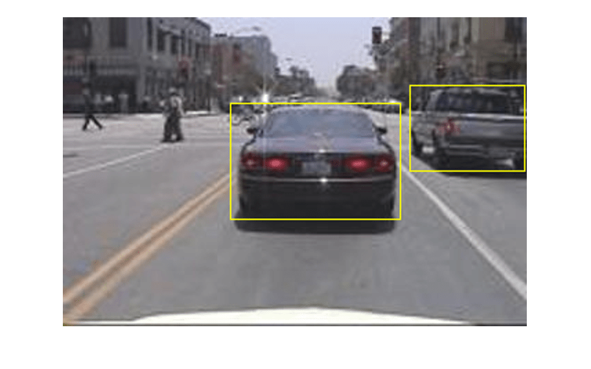
Create SSD Object Detection Network
Use the ssdObjectDetector function to automatically create an SSD object detector. The ssdObjectDetector function requires you to specify several inputs that parameterize the SSD object detector, including the base network (also known as feature extraction network), input size, class names, anchor boxes, and detection network sources. Use the specific layers from input base network to specify the detection network source. A detection network is automatically connected to the input base network by ssdObjectDetector function.
The feature extraction network is typically a pretrained CNN (see Pretrained Deep Neural Networks (Deep Learning Toolbox) for more details). This example uses ResNet-50 for feature extraction. Other pretrained networks such as MobileNet v2 or ResNet-18 can also be used depending on application requirements. The detection sub-network is a small CNN compared to the feature extraction network and is composed of a few convolutional layers and layers specific to SSD.
net = imagePretrainedNetwork("resnet50");When choosing the network input size, consider the size of the training images, and the computational cost incurred by processing data at the selected size. When feasible, choose a network input size that is close to the size of the training image. However, to reduce the computational cost of running this example, the network input size is chosen to be [300 300 3]. During training, trainSSDObjectDetector automatically resizes the training images to the network input size.
inputSize = [300 300 3];
Define object classes to detect.
classNames = "vehicle";This example modifies the pretrained ResNet-50 base network so that it is more robust. First, remove the layers in the ResNet-50 network present after the "activation_40_relu" layer. This also removes the fully connected layers. Then, add seven convolutional layers after the "activation_40_relu" layer to make the base network more robust.
% Find layer index of "activation_40_relu"
idx = find(ismember({net.Layers.Name},"activation_40_relu"));

% Remove all layers after "activation_40_relu" layer
removedLayers = {net.Layers(idx+1:end).Name};
ssdNet = removeLayers(net,removedLayers);

weightsInitializerValue = "glorot";
biasInitializerValue = "zeros";

% Append extra layers on top of a base network.
extraLayers = [];

% Add conv6_1 and corresponding reLU
filterSize = 1;
numFilters = 256;
numChannels = 1024;
conv6_1 = convolution2dLayer(filterSize,numFilters, ...
    NumChannels=numChannels, ...
    Name="conv6_1", ...
    WeightsInitializer=weightsInitializerValue, ...
    BiasInitializer=biasInitializerValue);
relu6_1 = reluLayer(Name="relu6_1");
extraLayers = [extraLayers; conv6_1; relu6_1];

% Add conv6_2 and corresponding reLU
filterSize = 3;
numFilters = 512;
numChannels = 256;
conv6_2 = convolution2dLayer(filterSize,numFilters, ...
    NumChannels=numChannels, ...
    Padding=iSamePadding(filterSize), ...
    Stride=[2 2], ...
    Name="conv6_2", ...
    WeightsInitializer=weightsInitializerValue, ...
    BiasInitializer=biasInitializerValue);
relu6_2 = reluLayer(Name="relu6_2");
extraLayers = [extraLayers; conv6_2; relu6_2];

% Add conv7_1 and corresponding reLU
filterSize = 1;
numFilters = 128;
numChannels = 512;
conv7_1 = convolution2dLayer(filterSize,numFilters, ...
    NumChannels=numChannels, ...
    Name="conv7_1", ...
    WeightsInitializer=weightsInitializerValue, ...
    BiasInitializer=biasInitializerValue);
relu7_1 = reluLayer(Name="relu7_1");
extraLayers = [extraLayers; conv7_1; relu7_1];

% Add conv7_2 and corresponding reLU
filterSize = 3;
numFilters = 256;
numChannels = 128;
conv7_2 = convolution2dLayer(filterSize,numFilters, ...
    NumChannels=numChannels, ...
    Padding=iSamePadding(filterSize), ...
    Stride=[2 2], ...
    Name="conv7_2", ...
    WeightsInitializer=weightsInitializerValue, ...
    BiasInitializer=biasInitializerValue);
relu7_2 = reluLayer(Name="relu7_2");
extraLayers = [extraLayers; conv7_2; relu7_2];

% Add conv8_1 and corresponding reLU
filterSize = 1;
numFilters = 128;
numChannels = 256;
conv8_1 = convolution2dLayer(filterSize,numFilters, ...
    NumChannels=numChannels, ...
    Name="conv8_1", ...
    WeightsInitializer=weightsInitializerValue, ...
    BiasInitializer=biasInitializerValue);
relu8_1 = reluLayer(Name="relu8_1");
extraLayers = [extraLayers; conv8_1; relu8_1];

% Add conv8_2 and corresponding reLU
filterSize = 3;
numFilters = 256;
numChannels = 128;
conv8_2 = convolution2dLayer(filterSize,numFilters, ...
    NumChannels=numChannels, ...
    Name="conv8_2", ...
    WeightsInitializer=weightsInitializerValue, ...
    BiasInitializer=biasInitializerValue);
relu8_2 = reluLayer(Name="relu8_2");
extraLayers = [extraLayers; conv8_2; relu8_2];

% Add conv9_1 and corresponding reLU
filterSize = 1;
numFilters = 128;
numChannels = 256;
conv9_1 = convolution2dLayer(filterSize,numFilters, ...
    NumChannels=numChannels, ...
    Padding=iSamePadding(filterSize), ...
    Name="conv9_1", ...
    WeightsInitializer=weightsInitializerValue, ...
    BiasInitializer=biasInitializerValue);
relu9_1 = reluLayer(Name="relu9_1");
extraLayers = [extraLayers; conv9_1; relu9_1];

if ~isempty(extraLayers)
    lastLayerName = ssdNet.Layers(end).Name;
    ssdNet = addLayers(ssdNet, extraLayers);
    ssdNet = connectLayers(ssdNet, lastLayerName, extraLayers(1).Name);
end
Note that the above changes are specific to the ResNet-50 backbone. It is possible to modify different backbones such as ResNet-101 or ResNet-18 to work with ssdObjectDetector. In order to do this, certain adjustments must be made to align directly with SSD's defined detection heads. To successfully modify these other networks, and using ResNet-101 as an example, first use analyzeNetwork(imagePretrainedNetwork("resnet101")).
There are numerous residual blocks (named res3a, res3b1... res4b2....res5b....) corresponding to different convolutional sizes. In order to correctly build an SSD object detector, the layers removed and the chosen detection heads should align with the SSD paper [1].
For ResNet-101, remove the layers after "res4b22_relu" and then use "res3b3_relu", "res4b22_relu", "relu6_2", "relu7_2", "relu8_2" as detection heads.
Specify the layers name from the network to which the detection network source will be added.
detNetworkSource = ["activation_22_relu", "activation_40_relu", "relu6_2", "relu7_2", "relu8_2"];
Specify the anchor boxes. The number of anchor boxes must be the same as the number of layers in the detection network source.
anchorBoxes = {[60,30;30,60;60,21;42,30]; ...
               [111,60;60,111;111,35;64,60;111,42;78,60]; ...
               [162,111;111,162;162,64;94,111;162,78;115,111]; ...
               [213,162;162,213;213,94;123,162;213,115;151,162]; ...
               [264,213;213,264;264,151;187,213]};
Create the SSD object detector object.
detector = ssdObjectDetector(ssdNet,classNames,anchorBoxes, ...
    DetectionNetworkSource=detNetworkSource,InputSize=inputSize,ModelName="ssdVehicle");
Data Augmentation
Data augmentation is used to improve network accuracy by randomly transforming the original data during training. By using data augmentation, you can add more variety to the training data without actually having to increase the number of labeled training samples. Use transform to augment the training data by
Randomly flipping the image and associated box labels horizontally.
Randomly scale the image, associated box labels.
Jitter image color.
Note that data augmentation is not applied to the test data. Ideally, test data should be representative of the original data and is left unmodified for unbiased evaluation.
augmentedTrainingData = transform(trainingData,@augmentData);
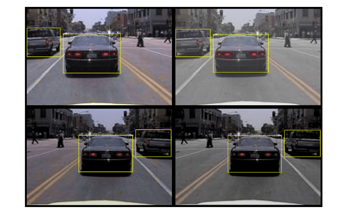
Visualize augmented training data by reading the same image multiple times.
augmentedData = cell(4,1);
for k = 1:4
    data = read(augmentedTrainingData);
    augmentedData{k} = insertShape(data{1},"rectangle",data{2});
    reset(augmentedTrainingData);
end

figure
montage(augmentedData,BorderSize=10)
Preprocess Training Data
Preprocess the augmented training data to prepare for training.
preprocessedTrainingData = transform(augmentedTrainingData, ...
    @(data)preprocessData(data,inputSize));
Read the preprocessed training data.
data = read(preprocessedTrainingData);
Display the image and bounding boxes.
I = data{1};
bbox = data{2};
annotatedImage = insertShape(I,"rectangle",bbox);
annotatedImage = imresize(annotatedImage,2);
figure
imshow(annotatedImage)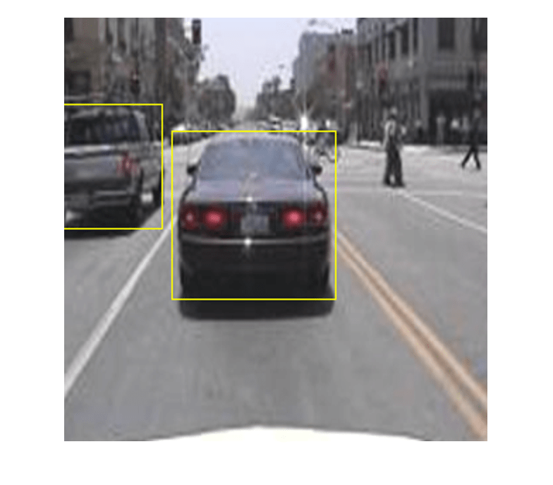
Train SSD Object Detector
Use trainingOptions to specify network training options. Set CheckpointPath to a temporary location. This enables the saving of partially trained detectors during the training process. If training is interrupted, such as by a power outage or system failure, you can resume training from the saved checkpoint.
options = trainingOptions("sgdm", ...
        MiniBatchSize=16, ....
        InitialLearnRate=1e-3, ...
        LearnRateSchedule="piecewise", ...
        LearnRateDropPeriod=30, ...
        LearnRateDropFactor=0.8, ...
        MaxEpochs=20, ...
        VerboseFrequency=50, ...
        CheckpointPath=tempdir, ...
        Shuffle="every-epoch");
If doTraining is true, then train the SSD object detector by using the trainSSDObjectDetector function. Otherwise, load a pretrained network.
if doTraining
    % Train the SSD detector.
    [detector,info] = trainSSDObjectDetector(preprocessedTrainingData,detector,options);
else
    % Load pretrained detector for the example.
    pretrained = load("ssdResNet50VehicleExample_22b.mat");
    detector = pretrained.detector;
end
Training this network takes approximately 2 hours using an NVIDIA™ Titan X GPU with 12 GB of memory. The training time varies depending on the hardware you use. If your GPU has less memory, you may run out of memory. If this happens, lower the MiniBatchSize using the trainingOptions function.
As a quick test, run the detector on one test image.
data = read(testData);
I = data{1,1};
I = imresize(I,inputSize(1:2));
[bboxes,scores] = detect(detector,I);
Display the results.
I = insertObjectAnnotation(I,"rectangle",bboxes,scores);
figure
imshow(I)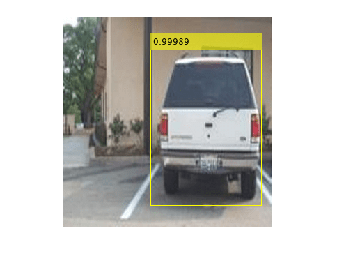
Evaluate Detector Using Test Set
Evaluate the trained object detector on a large set of images to measure the performance. Computer Vision Toolbox™ provides an object detector evaluation function (evaluateObjectDetection) to measure common metrics such as average precision and log-average miss rate. For this example, use the average precision metric to evaluate performance. The average precision provides a single number that incorporates the ability of the detector to make correct classifications (precision) and the ability of the detector to find all relevant objects (recall).
Apply the same preprocessing transform to the test data as for the training data. Note that data augmentation is not applied to the test data. Test data should be representative of the original data and be left unmodified for unbiased evaluation.
preprocessedTestData = transform(testData,@(data)preprocessData(data,inputSize));
Run the detector on all the test images. Set the detection threshold to a low value to detect as many objects as possible. This helps you evaluate the detector precision across the full range of recall values.
detectionThreshold = 0.01;
detectionResults = detect(detector,preprocessedTestData, ...
    Threshold=detectionThreshold,MiniBatchSize=32);
Evaluate the object detector using average precision metric.
metrics = evaluateObjectDetection(detectionResults,preprocessedTestData);
[precision,recall] = precisionRecall(metrics,ClassName="vehicle");
AP = averagePrecision(metrics,ClassName="vehicle");
The precision-recall (PR) curve highlights how precise a detector is at varying levels of recall. Ideally, the precision would be 1 at all recall levels. The use of more data can help improve the average precision, but might require more training time. Plot the PR curve.
figure
plot(recall{:},precision{:})
xlabel("Recall")
ylabel("Precision")
grid on
title("Average Precision = "+AP)
Code Generation
Once the detector is trained and evaluated, you can generate code for the ssdObjectDetector using GPU Coder™. For more details, see Code Generation for Object Detection by Using Single Shot Multibox Detector example.
Supporting Functions
function B = augmentData(A)
% Apply random horizontal flipping, and random X/Y scaling. Boxes that get
% scaled outside the bounds are clipped if the overlap is above 0.25. Also,
% jitter image color.
B = cell(size(A));
I = A{1};
sz = size(I);
if numel(sz)==3 && sz(3) == 3
    I = jitterColorHSV(I,...
        Contrast=0.2,...
        Hue=0,...
        Saturation=0.1,...
        Brightness=0.2);
end
% Randomly flip and scale image.
tform = randomAffine2d(XReflection=true,Scale=[1 1.1]);
rout = affineOutputView(sz,tform,BoundsStyle="CenterOutput");
B{1} = imwarp(I,tform,OutputView=rout);
% Sanitize boxes, if needed. This helper function is attached as a
% supporting file. Open the example in MATLAB to access this function.
A{2} = helperSanitizeBoxes(A{2});
% Apply same transform to boxes.
[B{2},indices] = bboxwarp(A{2},tform,rout,OverlapThreshold=0.25);
B{3} = A{3}(indices);
% Return original data only when all boxes are removed by warping.
if isempty(indices)
    B = A;
end
end

function data = preprocessData(data,targetSize)
% Resize image and bounding boxes to the targetSize.
sz = size(data{1},[1 2]);
scale = targetSize(1:2)./sz;
data{1} = imresize(data{1},targetSize(1:2));
% Sanitize boxes, if needed. This helper function is attached as a
% supporting file. Open the example in MATLAB to access this function.
data{2} = helperSanitizeBoxes(data{2});
% Resize boxes.
data{2} = bboxresize(data{2},scale);
end

function p = iSamePadding(FilterSize)
    p = floor(FilterSize / 2);
end
References
[1] Liu, Wei, Dragomir Anguelov, Dumitru Erhan, Christian Szegedy, Scott Reed, Cheng Yang Fu, and Alexander C. Berg. "SSD: Single shot multibox detector." In 14th European Conference on Computer Vision, ECCV 2016. Springer Verlag, 2016.
See Also
Apps
- Deep Network Designer (Deep Learning Toolbox)
Functions
estimateAnchorBoxes|analyzeNetwork(Deep Learning Toolbox) |combine|transform|read|evaluateObjectDetection