scatteringFeatures
Syntax
Description
concatenates the values of the dictionary of JTFS coefficients smat
= scatteringFeatures(jtfn
,cfs
)cfs
along the path dimension. cfs
is the output of scatteringTransform
.
specifies options using one or more name-value arguments. You can add these arguments to
either of the previous input syntaxes. For example, to exclude the second-order time
scattering coefficients with spin-up wavelets from the output, set
smat
= scatteringFeatures(___,Name=Value
)ExcludeCoefficients
to "SpinUp"
.
Note
Raw Data Input name-value
arguments are valid only for x
.
Examples
Create a single-precision random signal with three channels and 1024 samples representing one batch. Save the signal as a dlarray
in "CTB"
format.
nchan = 3;
nsam = 1024;
nbatch = 1;
sig = single(randn([nchan nsam nbatch]));
x = dlarray(sig,"CTB");
Create a JTFS network appropriate for the signal. Set the filter data type of the network to "single"
.
jtfn = timeFrequencyScattering(SignalLength=nsam, ... FilterDataType="single");
Use the scatteringTransform
function to obtain the JTFS transform of the signal. Specify a time oversampling factor of 1 and exclude the "S1SpinUpFreqLowpass"
coefficients.
tosf = 1; excl = "S1SpinUpFreqLowpass"; outCFS = scatteringTransform(jtfn,x, ... TimeOverSamplingFactor=tosf, ... ExcludeCoefficients=excl)
outCFS = dictionary (string ⟼ cell) with 4 entries: "S1FreqLowpass" ⟼ {1×6×16×3 dlarray} "SpinUp" ⟼ {35×6×16×3 dlarray} "SpinDown" ⟼ {35×6×16×3 dlarray} "U2JointLowpass" ⟼ {7×6×16×3 dlarray}
Use the same input arguments with the scatteringFeatures
function to obtain the JTFS coefficients as a tensor. Confirm the tensor is an unformatted dlarray
and the underlying data type is single precision.
smat = scatteringFeatures(jtfn,x, ... TimeOverSamplingFactor=tosf, ... ExcludeCoefficients=excl); size(smat)
ans = 1×4
78 6 16 3
dims(smat)
ans = 0×0 empty char array
underlyingType(smat)
ans = 'single'
Concatenate the dictionary values of outCFS
along the first (path) dimension. Confirm the result is equal to the tensor smat
.
dValues = values(outCFS); dValuesConCat = cat(1,dValues{:}); max(abs(smat(:)-dValuesConCat(:)))
ans = 1×1 single dlarray 0
Load a signal. Create a JTFS network appropriate for the signal.
load noisdopp
sig = noisdopp;
len = numel(sig);
jtfn = timeFrequencyScattering(SignalLength=len);
Use the scatteringFeatures
function to obtain the JTFS transform of the signal as a tensor. The result is a 3-D array with format path-by-frequency-by-time.
smatOrig = scatteringFeatures(jtfn,sig); size(smatOrig)
ans = 1×3
83 6 8
"zscore"
Normalization
Use the scatteringFeatures
function to apply the "zscore"
normalization method to the JTFS coefficients. When you specify this method, scatteringFeatures
normalizes the coefficients by subtracting the mean and dividing by the standard deviation across the frequency and time dimensions. For the standard deviation, the function uses the default weight of 0.
smatZscore = scatteringFeatures(jtfn,sig, ... Normalization="zscore");
Obtain the mean across the second (frequency) and third (time) dimensions of the array. The result is a vector whose length is the number of paths. Each vector element is the mean of the normalized JTFS coefficients on the corresponding path. Confirm the largest mean is approximately 0.
mn = mean(smatZscore,[2 3]); size(mn)
ans = 1×2
83 1
max(abs(mn))
ans = 1.7023e-15
Confirm the standard deviation of the normalized coefficients on each path is equal to 1.
stdCoef = std(smatZscore,[],[2 3]); [min(stdCoef) max(stdCoef)]
ans = 1×2
1.0000 1.0000
Use the zscore
(Statistics and Machine Learning Toolbox) function to obtain the z-scores of the original coefficients across the frequency and time dimensions. Confirm they are equal to the normalized coefficients.
smatOrigZscore = zscore(smatOrig,0,[2 3]); max(abs(smatOrigZscore(:)-smatZscore(:)))
ans = 0
"log"
Normalization
Use the scatteringFeatures
function to apply the "log"
normalization method to the JTFS coefficients. When you specify the "log"
method, scatteringFeatures
first applies a logarithmic transformation to the coefficients and then obtains the z-score.
smatLog = scatteringFeatures(jtfn,sig, ... Normalization="log");
A quantile-quantile plot shows quantiles of a data set plotted versus the theoretical quantile values from a Gaussian distribution. If the distribution of the data set is normal, then the data plot appears linear.
Use the qqplot
(Statistics and Machine Learning Toolbox) function to display quantile-quantile plots of the raw and normalized coefficients. The "log"
normalization method has transformed the coefficients distribution closer to a Gaussian distribution.
qqplot(smatOrig(:))
title("Without Log Normalization")
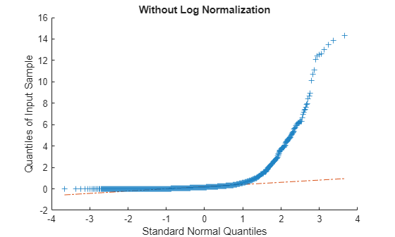
figure
qqplot(smatLog(:))
title("With Log Normalization")
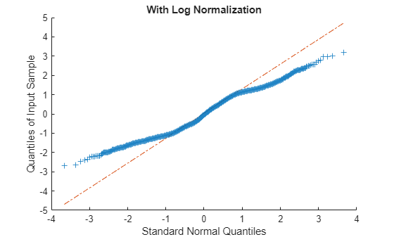
Input Arguments
Joint time-frequency scattering network, specified as a timeFrequencyScattering
object.
Input data, specified as a formatted or unformatted dlarray
(Deep Learning Toolbox) object
or a numeric array. If x
is a formatted dlarray
,
it must be in "CBT"
format. If x
is an
unformatted dlarray
, it must be compatible with
"CBT"
format and you must set
DataFormat
.
If x
is 2-D, the scatteringFeatures
function assumes the first dimension is time and the columns of x
are separate channels. If x
is 3-D, the dimensions of
x
are time-by-channel-by-batch.
If
x
is a vector or unformatteddlarray
, the number of samples inx
must match theSignalLength
property ofjtfn
.If
x
is a numeric or unformatted matrix or a 3-D array, the number of rows inx
must matchSignalLength
.If
x
is a formatteddlarray
, the length of the time dimension must matchSignalLength
.
Data Types: single
| double
JTFS coefficients, specified as a dictionary
object.
cfs
is the output of
scatteringTransform
.
Name-Value Arguments
Specify optional pairs of arguments as
Name1=Value1,...,NameN=ValueN
, where Name
is
the argument name and Value
is the corresponding value.
Name-value arguments must appear after other arguments, but the order of the
pairs does not matter.
Example: jtfs =
scatteringFeatures(jtfn,x,DataFormat="CBT",FrequencyAverage="global")
specifies
the format of the unformatted dlarray
x
as "CBT"
and takes the mean along the frequency
dimension for all JTFS coefficients.
All Inputs
Coefficients to exclude from the JTFS transform, specified as a string vector or cell array of character vectors. You can specify these coefficients:
"S1FreqLowpass"
— First-order time scattering coefficients filtered with the frequency lowpass filter"S1SpinUpFreqLowpass"
— First-order time scattering coefficients with the spin-up frequency wavelets"SpinUp"
— Second-order time scattering coefficients with spin-up wavelets"SpinDown"
— Second-order time scattering coefficients with spin-down wavelets"U2JointLowpass"
— Second-order time scattering coefficients filtered with joint lowpass filters
Example: jtfs =
scatteringFeatures(cfs,ExcludeCoefficients=["S1FreqLowpass"
"U2JointLowpass"])
Normalization method for JTFS coefficients, specified as one of the following:
"none"
— Do not normalize the coefficients."zscore"
— Subtract the mean and divide by the standard deviation across the frequency and time dimensions. For the standard deviation, thescatteringFeatures
function uses the default weight of 0."log"
— Logarithmic transformation followed by"zscore"
. This method transforms the JTFS coefficients distribution closer to a Gaussian distribution [1].
Raw Data Input
Time-averaging option, specified as one of these:
"local"
—scatteringFeatures
uses the lowpass filter when obtaining the JTFS coefficients."global"
—scatteringFeatures
takes the mean along the time dimension for all JTFS coefficients.
Frequency-averaging option, specified as one of these:
"local"
—scatteringFeatures
uses the lowpass frequency filter when obtaining the JTFS coefficients."global"
—scatteringFeatures
takes the mean along the frequency dimension for all JTFS coefficients.
Time oversampling factor, specified as a nonnegative integer. The factor specifies how much the coefficients are oversampled in time with respect to the critically downsampled values. The factor is on a base-2 logarithmic scale.
If you increase the oversampling factor, the computational costs and memory requirements of the scattering transform also increase.
Data Types: single
| double
Frequency oversampling factor, specified as a nonnegative integer. The factor specifies how much the coefficients are oversampled in frequency with respect to the critically downsampled values. The factor is on a base-2 logarithmic scale.
If you increase the oversampling factor, the computational costs and memory requirements of the scattering transform also increase.
Data Types: single
| double
Data format of x
, specified as a character vector or string
scalar. This name-value argument is valid only if x
is an
unformatted dlarray
. If x
is not a
dlarray
, DataFormat
is ignored.
Each character in this argument must be one of these labels:
"C"
— Channel"B"
— Batch observations"T"
— Time
DataFormat
can be any permutation of
"CBT"
.
Data Types: char
| string
Output Arguments
Joint time-frequency scattering transform, returned as an array or an unformatted
dlarray
object. If scatteringTransform
returns
the dictionary of JTFS coefficients outCFS
using a specific set of
input arguments, then scatteringFeatures
returns the concatenation
of those dictionary values using the same arguments.
References
[1] Lostanlen, Vincent, Christian El-Hajj, Mathias Rossignol, Grégoire Lafay, Joakim Andén, and Mathieu Lagrange. “Time–Frequency Scattering Accurately Models Auditory Similarities between Instrumental Playing Techniques.” EURASIP Journal on Audio, Speech, and Music Processing 2021, no. 1 (December 2021): 3. https://doi.org/10.1186/s13636-020-00187-z
Extended Capabilities
The scatteringFeatures
function
fully supports GPU arrays. To run the function on a GPU, specify the input data as a gpuArray
(Parallel Computing Toolbox). For more information, see Run MATLAB Functions on a GPU (Parallel Computing Toolbox).
Version History
Introduced in R2024b
MATLAB Command
You clicked a link that corresponds to this MATLAB command:
Run the command by entering it in the MATLAB Command Window. Web browsers do not support MATLAB commands.
Select a Web Site
Choose a web site to get translated content where available and see local events and offers. Based on your location, we recommend that you select: .
You can also select a web site from the following list
How to Get Best Site Performance
Select the China site (in Chinese or English) for best site performance. Other MathWorks country sites are not optimized for visits from your location.
Americas
- América Latina (Español)
- Canada (English)
- United States (English)
Europe
- Belgium (English)
- Denmark (English)
- Deutschland (Deutsch)
- España (Español)
- Finland (English)
- France (Français)
- Ireland (English)
- Italia (Italiano)
- Luxembourg (English)
- Netherlands (English)
- Norway (English)
- Österreich (Deutsch)
- Portugal (English)
- Sweden (English)
- Switzerland
- United Kingdom (English)