2-D Discrete Wavelet Analysis

This section takes you through the features of 2-D discrete wavelet analysis using the Wavelet Toolbox™ software. The toolbox provides these functions for image analysis. For more information, see the function reference pages.

Note

In this section the presentation and examples use 2-D arrays corresponding to indexed image representations. However, the functions described are also available when using truecolor images, which are represented by m-by-n-by-3 arrays of uint8.

Analysis-Decomposition Functions

Function Name	Purpose
dwt2	Single-level decomposition
wavedec2	Decomposition
wmaxlev	Maximum wavelet decomposition level

Synthesis-Reconstruction Functions

Function Name	Purpose
idwt2	Single-level reconstruction
waverec2	Full reconstruction
wrcoef2	Selective reconstruction
upcoef2	Single reconstruction

Decomposition Structure Utilities

Function Name	Purpose
detcoef2	Extraction of detail coefficients
appcoef2	Extraction of approximation coefficients
upwlev2	Recomposition of decomposition structure

Denoising and Compression

Function Name	Purpose
wdenoise2	Wavelet image denoising
ddencmp	Provide default values for denoising and compression
wbmpen	Penalized threshold for wavelet 1-D or 2-D denoising
wdcbm2	Thresholds for wavelet 2-D using Birgé-Massart strategy
wdencmp	Wavelet denoising and compression
wthrmngr	Threshold settings manager

In this section, you'll learn

• How to load an image

• How to analyze an image

• How to compress an image

Wavelet Image Analysis and Compression

This example shows how you can use 2-D wavelet analysis to compress an image efficiently without sacrificing its clarity.

Note: Instead of directly using image(I) to visualize the image I, we use image(wcodemat(I)), which displays a rescaled version of I leading to a clearer presentation of the details and approximations (see wcodemat).

Load an image.

load porche
whos X map

  Name        Size               Bytes  Class     Attributes

  X         512x512            2097152  double              
  map       235x3                 5640  double              

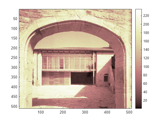
Display the image.

image(X)
colormap(map)
colorbar

If the colormap is smooth, the wavelet transform can be directly applied to the indexed image; otherwise the indexed image should be converted to grayscale format. For more information, see Wavelets: Working with Images. Since the colormap is smooth in this image, you can now perform the decomposition.

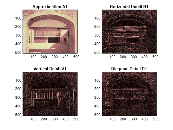
Perform a single-level wavelet decomposition of the image using the bior3.7 wavelet. The coefficient matrix cA1 are the approximation coefficients. The horizontal, vertical, and diagonal details are in the matrices cH1, cV1, and cD1, respectively.

wv = 'bior3.7';
[cA1,cH1,cV1,cD1] = dwt2(X,wv);

Use idwt1 to construct the approximations and details from the coefficients. (Note: You can also use upcoef2.)

sx = size(X);
A1 = idwt2(cA1,[],[],[],wv,sx);
H1 = idwt2([],cH1,[],[],wv,sx);
V1 = idwt2([],[],cV1,[],wv,sx);
D1 = idwt2([],[],[],cD1,wv,sx);

Display the approximations and details.

figure
tiledlayout(2,2)
nexttile
image(wcodemat(A1,192))
title('Approximation A1')
nexttile
image(wcodemat(H1,192))
title('Horizontal Detail H1')
nexttile
image(wcodemat(V1,192))
title('Vertical Detail V1')
nexttile
image(wcodemat(D1,192))
title('Diagonal Detail D1')
colormap(map)

Regenerate the image by the single-level inverse discrete wavelet transform. Confirm the difference between the regenerated and original images are small.

Xrec = idwt2(cA1,cH1,cV1,cD1,wv);
max(abs(X(:)-Xrec(:)))

ans = 
1.9895e-13

Perform a level-2 wavelet decomposition of the image using the same bior3.7 wavelet. The coefficients of all the components of a second-level decomposition (that is, the second-level approximation and the first two levels of detail) are returned concatenated into one vector, C. Argument S is a bookkeeping matrix that keeps track of the sizes of each component.

[c,s] = wavedec2(X,2,wv);

Extract the level 2 approximation coefficients. Extract the first- and second-level detail coefficients.

cA2 = appcoef2(c,s,wv,2);
[cH2,cV2,cD2] = detcoef2('all',c,s,2);
[cH1,cV1,cD1] = detcoef2('all',c,s,1);

Reconstruct the level 2 approximation and the level 1 and level 2 details.

A2 = wrcoef2('a',c,s,wv,2);
H1 = wrcoef2('h',c,s,wv,1);
V1 = wrcoef2('v',c,s,wv,1);
D1 = wrcoef2('d',c,s,wv,1);
H2 = wrcoef2('h',c,s,wv,2);
V2 = wrcoef2('v',c,s,wv,2);
D2 = wrcoef2('d',c,s,wv,2);

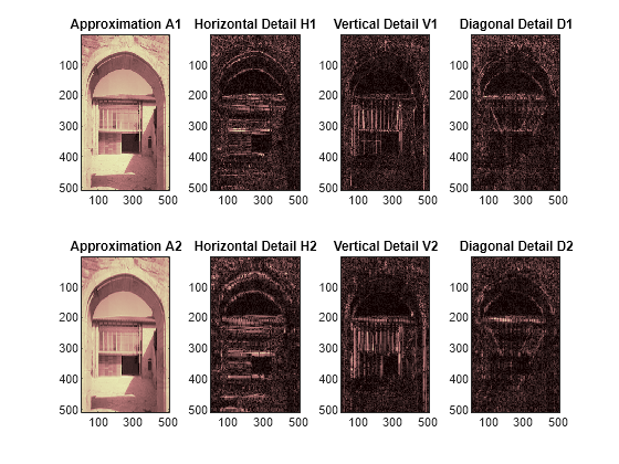
Display the approximation and details.

figure
tiledlayout(2,4)
nexttile
image(wcodemat(A1,192))
title('Approximation A1')
nexttile
image(wcodemat(H1,192))
title('Horizontal Detail H1')
nexttile
image(wcodemat(V1,192))
title('Vertical Detail V1')
nexttile
image(wcodemat(D1,192))
title('Diagonal Detail D1')
nexttile
image(wcodemat(A2,192))
title('Approximation A2')
nexttile
image(wcodemat(H2,192))
title('Horizontal Detail H2')
nexttile
image(wcodemat(V2,192))
title('Vertical Detail V2')
nexttile
image(wcodemat(D2,192))
title('Diagonal Detail D2')
colormap(map)

Compress the image. Use ddencmp to calculate the default parameters and wdencmp to perform the actual compression.

[thr,sorh,keepapp] = ddencmp('cmp','wv',X);
[Xcomp,CXC,LXC,PERF0,PERFL2] = ... 
wdencmp('gbl',c,s,wv,2,thr,sorh,keepapp);

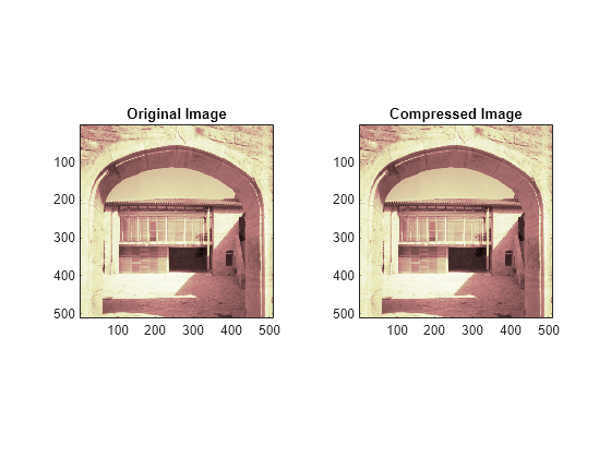
Compare the compressed image with the original image.

fprintf('Percentage of wavelet coefficients set to zero: %.4f\n',PERF0);

Percentage of wavelet coefficients set to zero: 52.2313

fprintf('Percentage of energy preserved: %.4f\n',PERFL2);

Percentage of energy preserved: 99.9982

figure
tiledlayout(1,2)
nexttile
image(X)
title('Original Image') 
axis square
nexttile
image(Xcomp)
title('Compressed Image') 
axis square
colormap(map)

Note that, even though the compressed image is constructed from only about half as many nonzero wavelet coefficients as the original, there is almost no detectable deterioration in the image quality.