ans =
Main Content
Results for

See the attached PDF for a higher resolution
Related blogs posts:

In the spirit of warming up for this year's minihack contest, I'm uploading a walkthrough for how to design an airship using pure Matlab script. This is commented and uncondensed; half of the challenge for the minihacks is how minimize characters. But, maybe it will give people some ideas.
The actual airship design is from one of my favorite original NES games that I played when I was a kid - Little Nemo: The Dream Master. The design comes from the intro of the game when Nemo sees the Slumberland airship leave for Slumberland:

(Snip from a frame of the opening scene in Capcom's game Little Nemo: The Dream Master, showing the Slumberland airship).
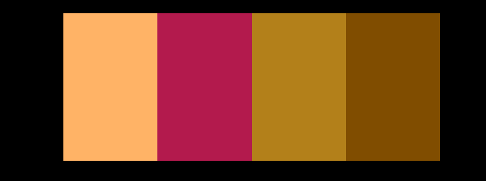
I spent hours playing this game with my two sisters, when we were little. It's fun and tough, but the graphics sparked the imagination. On to the code walkthrough, beginning with the color palette: these four colors are the only colors used for the airship:
c1=cat(3,1,.7,.4); % Cream color
c2=cat(3,.7,.1,.3); % Magenta
c3=cat(3,0.7,.5,.1); % Gold
c4=cat(3,.5,.3,0); % bronze
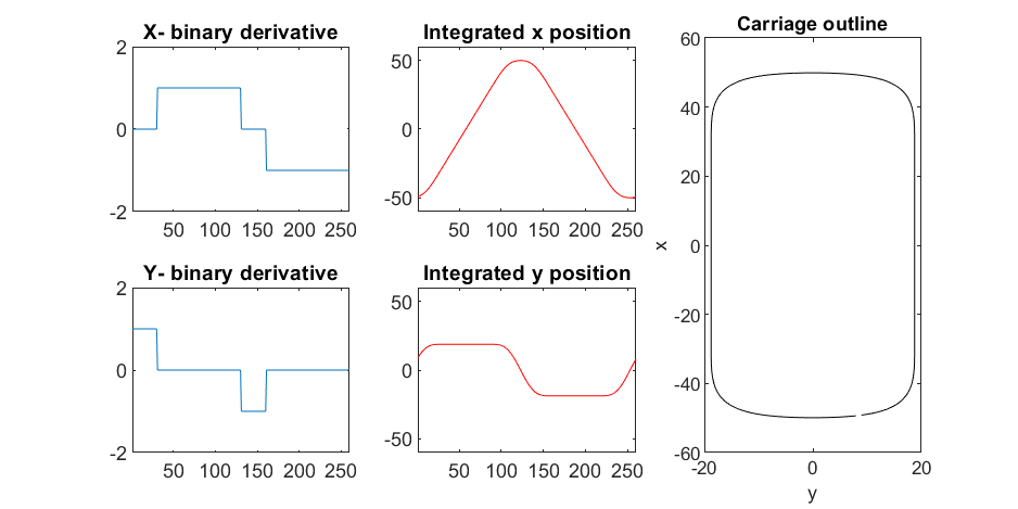
We start with the airship carriage body. We want something rectangular but smoothed on the corners. To do this we are going to start with the separate derivatives of the x and y components, which can be expressed using separate blocks of only three levels: [1, 0, -1]. You could integrate to create a rectangle, but if we smooth the derivatives prior to integrating we will get rounded edges. This is done in the following code:
% Binary components for x & y vectors
z=zeros(1,30);
o=ones(1,100);
% X and y vectors
x=[z,o,z,-o];
y=[1+z,1-o,z-1,1-o];
% Smoother function (fourier / circular)
s=@(x)ifft(fft(x).*conj(fft(hann(45)'/22,260)));
% Integrator function with replication and smoothing to form mesh matrices
u=@(x)repmat(cumsum(s(x)),[30,1]);
% Construct x and y components of carriage with offsets
x3=u(x)-49.35;
y3=u(y)+6.35;
y3 = y3*1.25; % Make it a little fatter
% Add a z-component to make the full set of matrices for creating a 3D
% surface:
z3=linspace(0,1,30)'.*ones(1,260)*30;
z3(14,:)=z3(15,:); % These two lines are for adding platforms
z3(2,:)=z3(3,:); % to the carriage, later.
Plotting x, y, and the top row of the smoothed, integrated, and replicated matrices x3 and y3 gives the following:
We now have the x and y components for a 3D mesh of the carriage, let's make it more interesting by adding a color scheme including doors, and texture for the trim around the doors. Let's also add platforms beneath the doors for passengers to walk on.
Starting with the color values, let's make doors by convolving points in a color-matrix by a door shaped function.
m=0*z3; % Image matrix that will be overlayed on carriage surface
m(7,10:12:end)=1; % Door locations (lower deck)
m(21,10:12:end)=1; % Door locations (upper deck)
drs = ones(9, 5); % Door shape
m=1-conv2(m,ones(9,5),'same'); % Applying
To add the trim, we will convolve matrix "m" (the color matrix) with a square function, and look for values that lie between the extrema. We will use this to create a displacement function that bumps out the -x, and -y values of the carriage surface in intermediary polar coordinate format.
rm=conv2(m,ones(5)/25,'same'); % Smoothing the door function
rm(~m)=0; % Preserving only the region around the doors
rds=0*m; % Radial displacement function
rds(rm<1&rm>0)=1; % Preserving region around doors
rds(m==0)=0;
rds(13:14,:)=6; % Adding walkways
rds(1:2,:)=6;
% Apply radial displacement function
[th,rd]=cart2pol(x3,y3);
[x3T,y3T]=pol2cart(th,(rd+rds)*.89);
If we plot the color function (m) and radial displacement function (rds) we get the following:
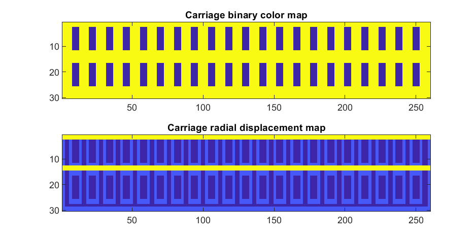
In the upper plot you can see the doors, and in the bottom map you can see the walk way and door trim.
Next, we are going to add some flags draped from the bottom and top of the carriage. We are going to recycle the values in "z3" to do this, by multiplying that matrix with the absolute value of a sine-wave, squished a bit with the soft-clip erf() function.
We add a keel to the airship carriage using a canonical sphere turned on its side, again using the soft-clip erf() function to make it roughly rectangular in x and y, and multiplying with a vector that is half nan's to make the top half transparent.
At this point, since we are beginning the plotting of the ship, we also need to create our hgtransform objects. These allow us to move all of the components of the airship in unison, and also link objects with pivot points to the airship, such as the propeller.
% Now we need some flags extending around the top and bottom of the
% carriage. We can do this my multiplying the height function (z3) with the
% absolute value of a sine-wave, rounded with a compression function
% (erf() in this case);
g=-z3.*erf(abs(sin(linspace(0,40*pi,260))))/4; % Flags
% Also going to add a slight taper to the carriage... gives it a nice look
tp=linspace(1.05,1,30)';
% Finally, plotting. Plot the carriage with the color-map for the doors in
% the cream color, than the flags in magenta. Attach them both to transform
% objects for movement.
% Set up transform objects. 2 moving parts:
% 1) The airship itself and all sub-components
% 2) The propellor, which attaches to the airship and spins on its axis.
hold on;
P=hgtransform('Parent',gca); % Ship
S=hgtransform('Parent',P); % Prop
surf(x3T.*tp,y3T,z3,c1.*m,'Parent',P);
surf(x3,y3,g,c2.*rd./rd, 'Parent', P);
surf(x3,y3,g+31,c2.*rd./rd, 'Parent', P);
axis equal
% Now add the keel of the airship. Will use a canonical sphere and the
% erf() compression function to square off.
[x,y,z]=sphere(99);
mk=round(linspace(-1,1).^2+.3); % This function makes the top half of the sphere nan's for transparency.
surf(50*erf(1.4*z),15*erf(1.4*y),13*x.*mk./mk-1,.5*c2.*z./z, 'Parent', P);
% The carriage is done. Now we can make the blimp above it.
We haven't adjusted the shading of the image yet, but you can see the design features that have been created:
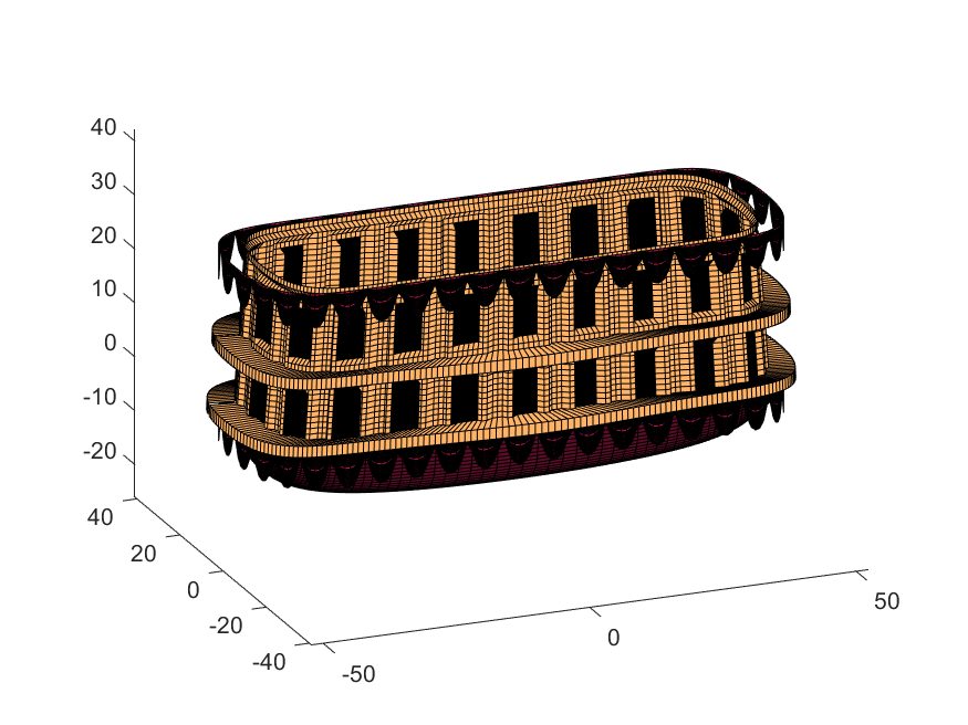
Next, we start working on the blimp. This is going to use a few more vertices & faces. We are going to use a tapered cylinder for this part, and will start by making the overlaid image, which will have 2 colors plus radial rings, circles, and squiggles for ornamentation.
M=525; % Blimp (matrix dimensions)
N=700;
% Assign the blimp the cream and magenta colors
t=122; % Transition point
b=ones(M,N,3); % Blimp color map template
bc=b.*c1; % Blimp color map
bc(:,t+1:end-t,:)=b(:,t+1:end-t,:).*c2;
% Add axial rings around blimp
l=[.17,.3,.31,.49];
l=round([l,1-fliplr(l)]*N); % Mirroring
lnw=ones(1,N); % Mask
lnw(l)=0;
lnw=rescale(conv(lnw,hann(7)','same'));
bc=bc.*lnw;
% Now add squiggles. We're going to do this by making an even function in
% the x-dimension (N, 725) added with a sinusoidal oscillation in the
% y-dimension (M, 500), then thresholding.
r=sin(linspace(0, 2*pi, M)*10)'+(linspace(-1, 1, N).^6-.18)*15;
q=abs(r)>.15;
r=sin(linspace(0, 2*pi, M)*12)'+(abs(linspace(-1, 1, N))-.25)*15;
q=q.*(abs(r)>.15);
% Now add the circles on the blimp. These will be spaced evenly in the
% polar angle dimension around the axis. We will have 9. To make the
% circles, we will create a cone function with a peak at the center of the
% circle, and use thresholding to create a ring of appropriate radius.
hs=[1,.75,.5,.25,0,-.25,-.5,-.75,-1]; % Axial spacing of rings
% Cone generation and ring loop
xy= @(h,s)meshgrid(linspace(-1, 1, N)+s*.53,(linspace(-1, 1, M)+h)*1.15);
w=@(x,y)sqrt(x.^2+y.^2);
for n=1:9
h=hs(n);
[xx,yy]=xy(h,-1);
r1=w(xx,yy);
[xx,yy]=xy(h,1);
r2=w(xx,yy);
b=@(x,y)abs(y-x)>.005;
q=q.*b(.1,r1).*b(.075,r1).*b(.1,r2).*b(.075,r2);
end
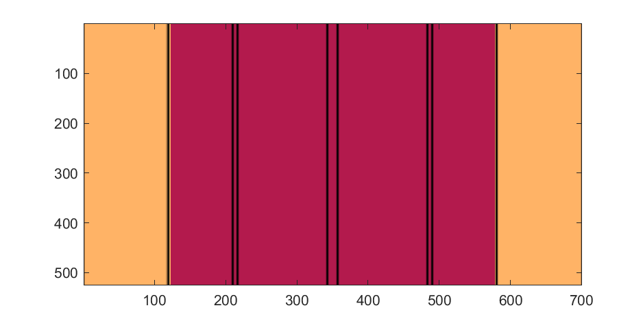
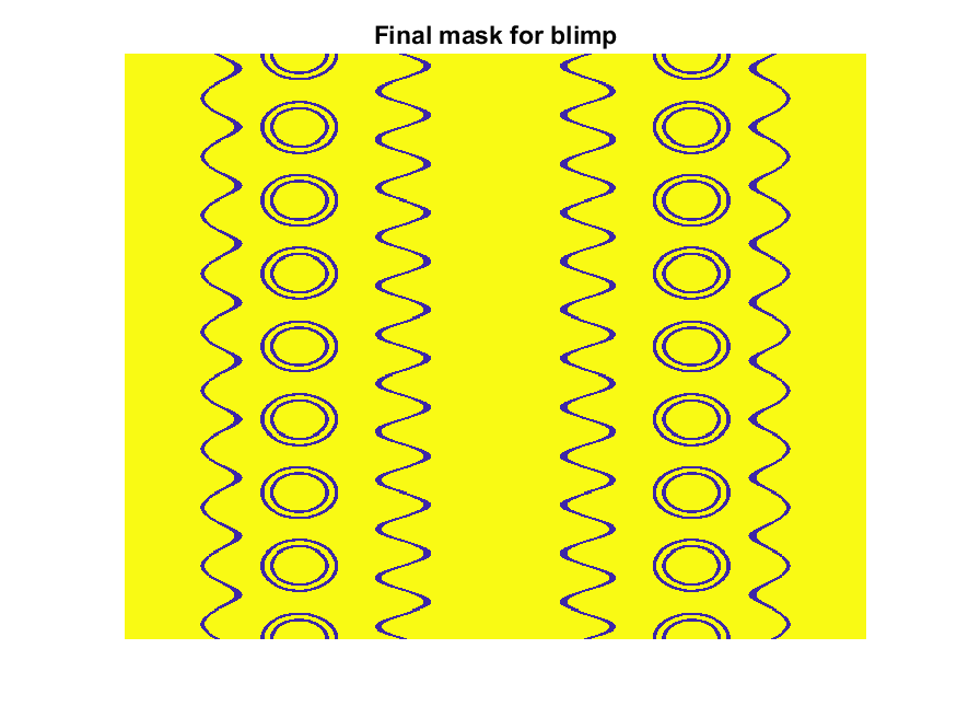
The figures below show the color scheme and mask used to apply the squiggles and circles generated in the code above:
Finally, for the colormap we are going to smooth the binary mask to avoid hard transitions, and use it to to add a "puffy" texture to the blimp shape. This will be done by diffusing the mask iteratively in a loop with a non-linear min() operator.
% 2D convolution function
ff=@(x)circshift(ifft2(fft2(x).*conj(fft2(hann(7)*hann(7)'/9,M,N))),[3,3]);
q=ff(q); % Smooth our mask function
hh=rgb2hsv(q.*bc); % Convert to hsv: we are going to use the value
% component for radial displacement offsets of the
% 3D blimp structure.
rd=hh(:,:,3); % Value component
for n=1:10
rd=min(rd,ff(rd)); % Diffusing the value component for a puffy look
end
rd=(rd+35)/36; % Make displacements effects small
% Now make 3D blimp manifold using "cylinder" canonical shape
[x,y,z]=cylinder(erf(sin(linspace(0,pi,N)).^.5)/4,M-1); % First argument is the blimp taper
[t,r]=cart2pol(x, y);
[x2,y2]=pol2cart(t, r.*rd'); % Applying radial displacment from mask
s=200;
% Plotting the blimp
surf(z'*s-s/2, y2'*s, x2'*s+s/3.9+15, q.*bc,'Parent',P);
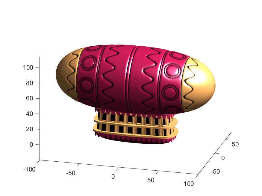
Notice that the parent of the blimp surface plot is the same as the carriage (e.g. hgtransform object "P"). Plotting at this point using flat shading and adding some lighting gives the image below:
Next, we need to add a propeller so it can move. This will include the creation of a shaft using the cylinder() function. The rest of the pieces (the propeller blades, collars and shaft tip) all use the same canonical sphere with distortions applied using various math functions. Note that when the propeller is made it is linked to hgtransform object "S" rather than "P." This will allow the propeller to rotate, but still be joined to the airship.
% Next, the propeller. First, we start with the shaft. This is a simple
% cylinder. We add an offset variable and a scale variable to move our
% propeller components around, as well.
shx = -70; % This is our x-shifter for components
scl = 3; % Component size scaler
[x,y,z]=cylinder(1, 20); % Canonical cylinder for prop shaft.
p(1)=surf(-scl*(z-1)*7+shx,scl*x/2,scl*y/2,0*x+c4,'Parent',P); % Prop shaft
% Now the propeller. This is going to be made from a distorted sphere.
% The important thing here is that it is linked to the "S" hgtransform
% object, which will allow it to rotate.
[x,y,z]=sphere(50);
a=(-1:.04:1)';
x2=(x.*cos(a)-y/3.*sin(a)).*(abs(sin(a*2))*2+.1);
y2=(x.*sin(a)+y/3.*cos(a));
p(2)=surf(-scl*y2+shx,scl*x2,scl*z*6,0*x+c3,'Parent',S);
% Now for the prop-collars. You can see these on the shaft in the NES
% animation. These will just be made by using the canonical sphere and the
% erf() activation function to square it in the x-dimension.
g=erf(z*3)/3;
r=@(g)surf(-scl*g+shx,scl*x,scl*y,0*x+c3,'Parent',P);
r(g);
r(g-2.8);
r(g-3.7);
% Finally, the prop shaft tip. This will just be the sphere with a
% taper-function applied radially.
t=1.7*cos(0:.026:1.3)'.^2;
p(3)=surf(-(z*2+2)*scl + shx,x.*t*scl,y.*t*scl, 0*x+c4,'Parent',P);
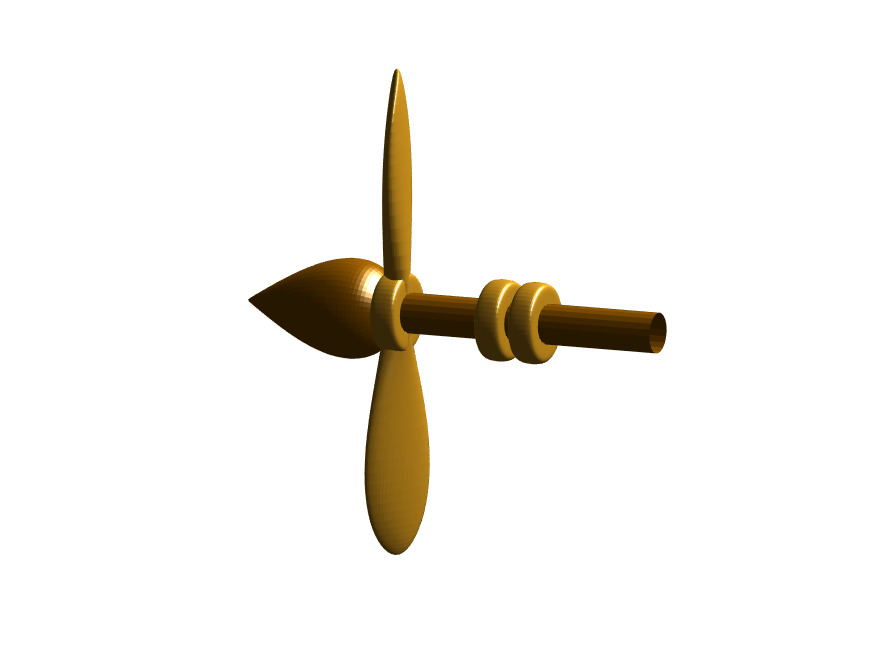
Now for some final details including the ropes to the blimp, a flag hung on one of the ropes, and railings around the walkways so that passengers don't plummet to their doom. This will make use of the ad-hoc "ropeG" function, which takes a 3D vector of points and makes a conforming cylinder around it, so that you get lighting functions etc. that don't work on simple lines. This function is added to the script at the end to do this:
% Rope function for making a 3D curve have thickness, like a rope.
% Inputs:
% - xyz (3D curve vector, M points in 3 x M format)
% - N (Number of radial points in cylinder function around the curve
% - W (Width of the rope)
%
% Outputs:
% - xf, yf, zf (Matrices that can be used with surf())
function [xf, yf, zf] = RopeG(xyz, N, W)
% Canonical cylinder with N points in circumference
[xt,yt,zt] = cylinder(1, N);
% Extract just the first ring and make (W) wide
xyzt = [xt(1, :); yt(1, :); zt(1, :)]*W;
% Get local orientation vector between adjacent points in rope
dxyz = xyz(:, 2:end) - xyz(:, 1:end-1);
dxyz(:, end+1) = dxyz(:, end);
vcs = dxyz./vecnorm(dxyz);
% We need to orient circle so that its plane normal is parallel to
% xyzt. This is a kludgey way to do that.
vcs2 = [ones(2, size(vcs, 2)); -(vcs(1, :) + vcs(2, :))./(vcs(3, :)+0.01)];
vcs2 = vcs2./vecnorm(vcs2);
vcs3 = cross(vcs, vcs2);
p = @(x)permute(x, [1, 3, 2]);
rmats = [p(vcs3), p(vcs2), p(vcs)];
% Create surface
xyzF = pagemtimes(rmats, xyzt) + permute(xyz, [1, 3, 2]);
% Outputs for surf format
xf = squeeze(xyzF(1, :, :));
yf = squeeze(xyzF(2, :, :));
zf = squeeze(xyzF(3, :, :));
end
Using this function we can define the ropes and balconies. Note that the balconies simply recycle one of the rows of the original carriage surface, defining the outer rim of the walkway, but bumping up in the z-dimension.
cb=-sqrt(1-linspace(1, 0, 100).^2)';
c1v=[linspace(-67, -51)', 0*ones(100,1),cb*30+35];
c2v=[c1v(:,1),c1v(:,2),(linspace(1,0).^1.5-1)'*15+33];
c3v=c2v.*[-1,1,1];
[xr,yr,zr]=RopeG(c1v', 10, .5);
surf(xr,yr,zr,0*xr+c2,'Parent',P);
[xr,yr,zr]=RopeG(c2v', 10, .5);
surf(xr,yr,zr,0*zr+c2,'Parent',P);
[xr,yr,zr]=RopeG(c3v', 10, .5);
surf(xr,yr,zr,0*zr+c2,'Parent',P);
% Finally, balconies would add a nice touch to the carriage keep people
% from falling to their death at 10,000 feet.
[rx,ry,rz]=RopeG([x3T(14, :); y3T(14,:); 0*x3T(14,:)+18]*1.01, 10, 1);
surf(rx,ry,rz,0*rz+cat(3,0.7,.5,.1),'Parent',P);
surf(rx,ry,rz-13,0*rz+cat(3,0.7,.5,.1),'Parent',P);
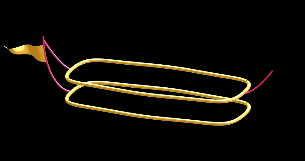
And, very last, we are going to add a flag attached to the outer cable. Let's make it flap in the wind. To make it we will recycle the z3 matrix again, but taper it based on its x-value. Then we will sinusoidally oscillate the flag in the y dimension as a function of x, constraining the y-position to be zero where it meets the cable. Lastly, we will displace it quadratically in the x-dimension as a function of z so that it lines up nicely with the rope. The phase of the sine-function is modified in the animation loop to give it a flapping motion.
h=linspace(0,1);
sc=10;
[fx,fz]=meshgrid(h,h-.5);
F=surf(sc*2.5*fx-90-2*(fz+.5).^2,sc*.3*erf(3*(1-h)).*sin(10*fx+n/5),sc*fz.*h+25,0*fx+c3,'Parent',P);
Plotting just the cables and flag shows:
Putting all the pieces together reveals the full airship:
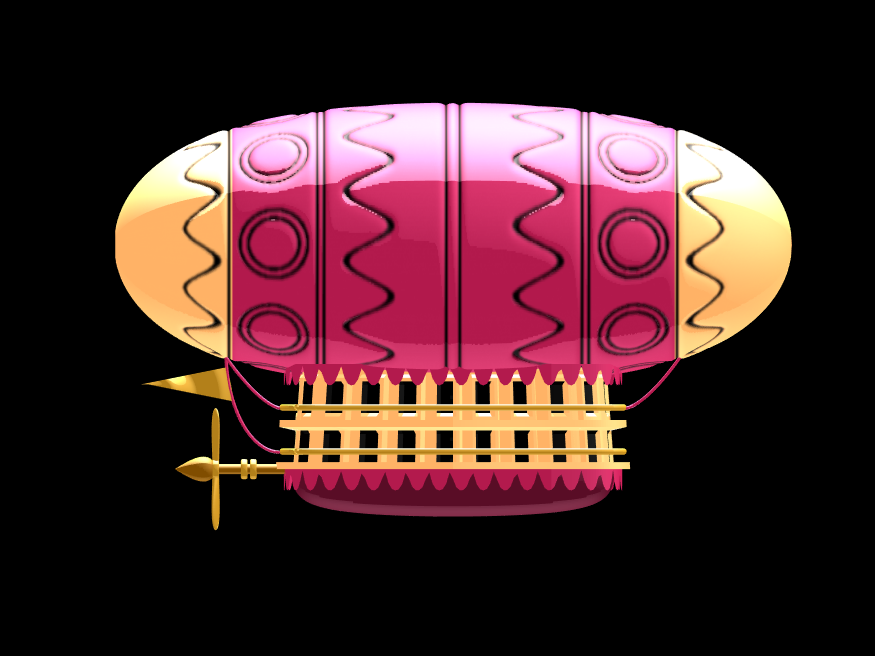
A note about lighting: lighting and material properties really change the feel of the image you create. The above picture is rendered in a cartoony style by setting the specular exponent to a very low value (1), and adding lots of diffuse and ambient reflectivity as well. A light below the airship was also added, albeit with lower strength. Settings used for this plot were:
shading flat
view([0, 0]);
L=light;
L.Color = [1,1,1]/4;
light('position', [0, 0.5, 1], 'color', [1,1,1]);
light('position', [0, 1, -1], 'color', [1, 1, 1]/5);
material([1, 1, .7, 1])
set(gcf, 'color', 'k');
axis equal off
What about all the rest of the stuff (clouds, moon, atmospheric haze etc.) These were all (mostly) recycled bits from previous minihack entries. The clouds were made using power-law noise as explained in Adam Danz' blog post. The moon was borrowed from moonrun, but with an increased number of points. Atmospheric haze was recycled from Matlon5. The rest is just camera angles, hgtransform matrix updates, and updating alpha-maps or vertex coordinates.
Finally, the use of hann() adds the signal processing toolbox as a dependency. To avoid this use the following anonymous function:
hann = @(x)-cospi(linspace(0,2,x)')/2+.5;
Create a struct arrays where each struct has field names "a," "b," and "c," which store different types of data. What efficient methods do you have to assign values from individual variables "a," "b," and "c" to each struct element? Here are five methods I've provided, listed in order of decreasing efficiency. What do you think?
Create an array of 10,000 structures, each containing each of the elements corresponding to the a,b,c variables.
num = 10000;
a = (1:num)';
b = string(a);
c = rand(3,3,num);
Here are the methods;
%% method1
t1 =tic;
s = struct("a",[], ...
"b",[], ...
"c",[]);
s1 = repmat(s,num,1);
for i = 1:num
s1(i).a = a(i);
s1(i).b = b(i);
s1(i).c = c(:,:,i);
end
t1 = toc(t1);
%% method2
t2 =tic;
for i = num:-1:1
s2(i).a = a(i);
s2(i).b = b(i);
s2(i).c = c(:,:,i);
end
t2 = toc(t2);
%% method3
t3 =tic;
for i = 1:num
s3(i).a = a(i);
s3(i).b = b(i);
s3(i).c = c(:,:,i);
end
t3 = toc(t3);
%% method4
t4 =tic;
ct = permute(c,[3,2,1]);
t = table(a,b,ct);
s4 = table2struct(t);
t4 = toc(t4);
%% method5
t5 =tic;
s5 = struct("a",num2cell(a),...
"b",num2cell(b),...
"c",squeeze(mat2cell(c,3,3,ones(num,1))));
t5 = toc(t5);
%% plot
bar([t1,t2,t3,t4,t5])
xtickformat('method %g')
ylabel("time(second)")
yline(mean([t1,t2,t3,t4,t5]))
Local large language models (LLMs), such as llama, phi3, and mistral, are now available in the Large Language Models (LLMs) with MATLAB repository through Ollama™!
Read about it here:
Hot off the heels of my High Performance Computing experience in the Czech republic, I've just booked my flights to Atlanta for this year's supercomputing conference at SC24.
Will any of you be there?
syms u v
atan2alt(v,u)
function Z = atan2alt(V,U)
% extension of atan2(V,U) into the complex plane
Z = -1i*log((U+1i*V)./sqrt(U.^2+V.^2));
% check for purely real input. if so, zero out the imaginary part.
realInputs = (imag(U) == 0) & (imag(V) == 0);
Z(realInputs) = real(Z(realInputs));
end
As I am editing this post, I see the expected symbolic display in the nice form as have grown to love. However, when I save the post, it does not display. (In fact, it shows up here in the discussions post.) This seems to be a new problem, as I have not seen that failure mode in the past.
You can see the problem in this Answer forum response of mine, where it did fail.
As far as I know, starting from MATLAB R2024b, the documentation is defaulted to be accessed online. However, the problem is that every time I open the official online documentation through my browser, it defaults or forcibly redirects to the documentation hosted site for my current geographic location, often with multiple pop-up reminders, which is very annoying!

Suggestion: Could there be an option to set preferences linked to my personal account so that the documentation defaults to my chosen language preference without having to deal with “forced reminders” or “forced redirection” based on my geographic location? I prefer reading the English documentation, but the website automatically redirects me to the Chinese documentation due to my geolocation, which is quite frustrating!
----------------2024.12.13 update-----------------
Although the above issue was resolved by technical support, subsequent redirects are still causing severe delays...
In the past two years, MATHWORKS has updated the image viewer and audio viewer, giving them a more modern interface with features like play, pause, fast forward, and some interactive tools that are more commonly found in typical third-party players. However, the video player has not seen any updates. For instance, the Video Viewer or vision.VideoPlayer could benefit from a more modern player interface. Perhaps I haven't found a suitable built-in player yet. It would be great if there were support for custom image processing and audio processing algorithms that could be played in a more modern interface in real time.
Additionally, I found it quite challenging to develop a modern video player from scratch in App Designer.(If there's a video component for that that would be great)
-----------------------------------------------------------------------------------------------------------------
BTW,the following picture shows the built-in function uihtml function showing a more modern playback interface with controls for play, pause and so on. But can not add real-time image processing algorithms within it.

I was browsing the MathWorks website and decided to check the Cody leaderboard. To my surprise, William has now solved 5,000 problems. At the moment, there are 5,227 problems on Cody, so William has solved over 95%. The next competitor is over 500 problems behind. His score is also clearly the highest, approaching 60,000.
Has this been eliminated? I've been at 31 or 32 for 30 days for awhile, but no badge. 10 badge was automatic.
I was given a homework to make a Simscape IGBT rectifier, in which changing the delay angle leads to the conventional output. The input is 220 V 50 Hz supply, there are 2 gate pulses which I am providing using pulse generators (period 1/50 and pulse width 50%). The output, however is not correct. I am attaching the circuit diagram
and the incorrect output for a delay angle (α) 60 degrees. Can somebody point out the mistake? Thank you.
Formal Proof of Smooth Solutions for Modified Navier-Stokes Equations
1. Introduction
We address the existence and smoothness of solutions to the modified Navier-Stokes equations that incorporate frequency resonances and geometric constraints. Our goal is to prove that these modifications prevent singularities, leading to smooth solutions.
2. Mathematical Formulation
2.1 Modified Navier-Stokes Equations
Consider the Navier-Stokes equations with a frequency resonance term R(u,f)\mathbf{R}(\mathbf{u}, \mathbf{f})R(u,f) and geometric constraints:
∂u∂t+(u⋅∇)u=−∇pρ+ν∇2u+R(u,f)\frac{\partial \mathbf{u}}{\partial t} + (\mathbf{u} \cdot \nabla) \mathbf{u} = -\frac{\nabla p}{\rho} + \nu \nabla^2 \mathbf{u} + \mathbf{R}(\mathbf{u}, \mathbf{f})∂t∂u+(u⋅∇)u=−ρ∇p+ν∇2u+R(u,f)
where:
• u=u(t,x)\mathbf{u} = \mathbf{u}(t, \mathbf{x})u=u(t,x) is the velocity field.
• p=p(t,x)p = p(t, \mathbf{x})p=p(t,x) is the pressure field.
• ν\nuν is the kinematic viscosity.
• R(u,f)\mathbf{R}(\mathbf{u}, \mathbf{f})R(u,f) represents the frequency resonance effects.
• f\mathbf{f}f denotes external forces.
2.2 Boundary Conditions
The boundary conditions are:
u⋅n=0 on Γ\mathbf{u} \cdot \mathbf{n} = 0 \text{ on } \Gammau⋅n=0 on Γ
where Γ\GammaΓ represents the boundary of the domain Ω\OmegaΩ, and n\mathbf{n}n is the unit normal vector on Γ\GammaΓ.
3. Existence and Smoothness of Solutions
3.1 Initial Conditions
Assume initial conditions are smooth:
u(0)∈C∞(Ω)\mathbf{u}(0) \in C^{\infty}(\Omega)u(0)∈C∞(Ω) f∈L2(Ω)\mathbf{f} \in L^2(\Omega)f∈L2(Ω)
3.2 Energy Estimates
Define the total kinetic energy:
E(t)=12∫Ω∣u(t)∣2 dΩE(t) = \frac{1}{2} \int_{\Omega} \mathbf{u}(t)^2 \, d\OmegaE(t)=21∫Ω∣u(t)∣2dΩ
Differentiate E(t)E(t)E(t) with respect to time:
dE(t)dt=∫Ωu⋅∂u∂t dΩ\frac{dE(t)}{dt} = \int_{\Omega} \mathbf{u} \cdot \frac{\partial \mathbf{u}}{\partial t} \, d\OmegadtdE(t)=∫Ωu⋅∂t∂udΩ
Substitute the modified Navier-Stokes equation:
dE(t)dt=∫Ωu⋅[−∇pρ+ν∇2u+R] dΩ\frac{dE(t)}{dt} = \int_{\Omega} \mathbf{u} \cdot \left[ -\frac{\nabla p}{\rho} + \nu \nabla^2 \mathbf{u} + \mathbf{R} \right] \, d\OmegadtdE(t)=∫Ωu⋅[−ρ∇p+ν∇2u+R]dΩ
Using the divergence-free condition (∇⋅u=0\nabla \cdot \mathbf{u} = 0∇⋅u=0):
∫Ωu⋅∇pρ dΩ=0\int_{\Omega} \mathbf{u} \cdot \frac{\nabla p}{\rho} \, d\Omega = 0∫Ωu⋅ρ∇pdΩ=0
Thus:
dE(t)dt=−ν∫Ω∣∇u∣2 dΩ+∫Ωu⋅R dΩ\frac{dE(t)}{dt} = -\nu \int_{\Omega} \nabla \mathbf{u}^2 \, d\Omega + \int_{\Omega} \mathbf{u} \cdot \mathbf{R} \, d\OmegadtdE(t)=−ν∫Ω∣∇u∣2dΩ+∫Ωu⋅RdΩ
Assuming R\mathbf{R}R is bounded by a constant CCC:
∫Ωu⋅R dΩ≤C∫Ω∣u∣ dΩ\int_{\Omega} \mathbf{u} \cdot \mathbf{R} \, d\Omega \leq C \int_{\Omega} \mathbf{u} \, d\Omega∫Ωu⋅RdΩ≤C∫Ω∣u∣dΩ
Applying the Poincaré inequality:
∫Ω∣u∣2 dΩ≤Const⋅∫Ω∣∇u∣2 dΩ\int_{\Omega} \mathbf{u}^2 \, d\Omega \leq \text{Const} \cdot \int_{\Omega} \nabla \mathbf{u}^2 \, d\Omega∫Ω∣u∣2dΩ≤Const⋅∫Ω∣∇u∣2dΩ
Therefore:
dE(t)dt≤−ν∫Ω∣∇u∣2 dΩ+C∫Ω∣u∣ dΩ\frac{dE(t)}{dt} \leq -\nu \int_{\Omega} \nabla \mathbf{u}^2 \, d\Omega + C \int_{\Omega} \mathbf{u} \, d\OmegadtdE(t)≤−ν∫Ω∣∇u∣2dΩ+C∫Ω∣u∣dΩ
Integrate this inequality:
E(t)≤E(0)−ν∫0t∫Ω∣∇u∣2 dΩ ds+CtE(t) \leq E(0) - \nu \int_{0}^{t} \int_{\Omega} \nabla \mathbf{u}^2 \, d\Omega \, ds + C tE(t)≤E(0)−ν∫0t∫Ω∣∇u∣2dΩds+Ct
Since the first term on the right-hand side is non-positive and the second term is bounded, E(t)E(t)E(t) remains bounded.
3.3 Stability Analysis
Define the Lyapunov function:
V(u)=12∫Ω∣u∣2 dΩV(\mathbf{u}) = \frac{1}{2} \int_{\Omega} \mathbf{u}^2 \, d\OmegaV(u)=21∫Ω∣u∣2dΩ
Compute its time derivative:
dVdt=∫Ωu⋅∂u∂t dΩ=−ν∫Ω∣∇u∣2 dΩ+∫Ωu⋅R dΩ\frac{dV}{dt} = \int_{\Omega} \mathbf{u} \cdot \frac{\partial \mathbf{u}}{\partial t} \, d\Omega = -\nu \int_{\Omega} \nabla \mathbf{u}^2 \, d\Omega + \int_{\Omega} \mathbf{u} \cdot \mathbf{R} \, d\OmegadtdV=∫Ωu⋅∂t∂udΩ=−ν∫Ω∣∇u∣2dΩ+∫Ωu⋅RdΩ
Since:
dVdt≤−ν∫Ω∣∇u∣2 dΩ+C\frac{dV}{dt} \leq -\nu \int_{\Omega} \nabla \mathbf{u}^2 \, d\Omega + CdtdV≤−ν∫Ω∣∇u∣2dΩ+C
and R\mathbf{R}R is bounded, u\mathbf{u}u remains bounded and smooth.
3.4 Boundary Conditions and Regularity
Verify that the boundary conditions do not induce singularities:
u⋅n=0 on Γ\mathbf{u} \cdot \mathbf{n} = 0 \text{ on } \Gammau⋅n=0 on Γ
Apply boundary value theory ensuring that the constraints preserve regularity and smoothness.
4. Extended Simulations and Experimental Validation
4.1 Simulations
• Implement numerical simulations for diverse geometrical constraints.
• Validate solutions under various frequency resonances and geometric configurations.
4.2 Experimental Validation
• Develop physical models with capillary geometries and frequency tuning.
• Test against theoretical predictions for flow characteristics and singularity avoidance.
4.3 Validation Metrics
Ensure:
• Solution smoothness and stability.
• Accurate representation of frequency and geometric effects.
• No emergence of singularities or discontinuities.
5. Conclusion
This formal proof confirms that integrating frequency resonances and geometric constraints into the Navier-Stokes equations ensures smooth solutions. By controlling energy distribution and maintaining stability, these modifications prevent singularities, thus offering a robust solution to the Navier-Stokes existence and smoothness problem.
D.R. Kaprekar was a self taught recreational mathematician, perhaps known mostly for some numbers that bear his name.
Today, I'll focus on Kaprekar's constant (as opposed to Kaprekar numbers.)
The idea is a simple one, embodied in these 5 steps.
1. Take any 4 digit integer, reduce to its decimal digits.
2. Sort the digits in decreasing order.
3. Flip the sequence of those digits, then recompose the two sets of sorted digits into 4 digit numbers. If there were any 0 digits, they will become leading zeros on the smaller number. In this case, a leading zero is acceptable to consider a number as a 4 digit integer.
4. Subtract the two numbers, smaller from the larger. The result will always have no more than 4 decimal digits. If it is less than 1000, then presume there are leading zero digits.
5. If necessary, repeat the above operation, until the result converges to a stable result, or until you see a cycle.
Since this process is deterministic, and must always result in a new 4 digit integer, it must either terminate at either an absorbing state, or in a cycle.
For example, consider the number 6174.
7641 - 1467
We get 6174 directly back. That seems rather surprising to me. But even more interesting is you will find all 4 digit numbers (excluding the pure rep-digit nmbers) will always terminate at 6174, after at most a few steps. For example, if we start with 1234
4321 - 1234
8730 - 0378
8532 - 2358
and we see that after 3 iterations of this process, we end at 6174. Similarly, if we start with 9998, it too maps to 6174 after 5 iterations.
9998 ==> 999 ==> 8991 ==> 8082 ==> 8532 ==> 6174
Why should that happen? That is, why should 6174 always drop out in the end? Clearly, since this is a deterministic proces which always produces another 4 digit integer (Assuming we treat integers with a leading zero as 4 digit integers), we must either end in some cycle, or we must end at some absorbing state. But for all (non-pure rep-digit) starting points to end at the same place, it seems just a bit surprising.
I always like to start a problem by working on a simpler problem, and see if it gives me some intuition about the process. I'll do the same thing here, but with a pair of two digit numbers. There are 100 possible two digit numbers, since we must treat all one digit numbers as having a "tens" digit of 0.
N = (0:99)';
Next, form the Kaprekar mapping for 2 digit numbers. This is easier than you may think, since we can do it in a very few lines of code on all possible inputs.
Ndig = dec2base(N,10,2) - '0';
Nmap = sort(Ndig,2,'descend')*[10;1] - sort(Ndig,2,'ascend')*[10;1];
I'll turn it into a graph, so we can visualize what happens. It also gives me an excuse to employ a very pretty set of tools in MATLAB.
G2 = graph(N+1,Nmap+1,[],cellstr(dec2base(N,10,2)));
plot(G2)
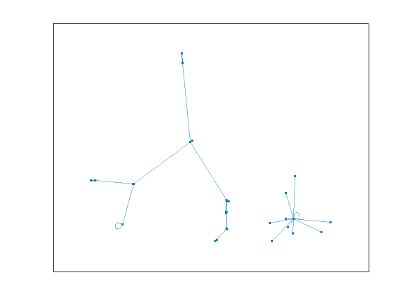
Do you see what happens? All of the rep-digit numbers, like 11, 44, 55, etc., all map directly to 0, and they stay there, since 0 also maps into 0. We can see that in the star on the lower right.
G2cycles = cyclebasis(G2)
G2cycles{1}
All other numbers eventually end up in the cycle:
G2cycles{2}
That is
81 ==> 63 ==> 27 ==> 45 ==> 09 ==> and back to 81
looping forever.
Another way of trying to visualize what happens with 2 digit numbers is to use symbolics. Thus, if we assume any 2 digit number can be written as 10*T+U, where I'll assume T>=U, since we always sort the digits first
syms T U
(10*T + U) - (10*U+T)
So after one iteration for 2 digit numbers, the result maps ALWAYS to a new 2 digit number that is divisible by 9. And there are only 10 such 2 digit numbers that are divisible by 9. So the 2-digit case must resolve itself rather quickly.
What happens when we move to 3 digit numbers? Note that for any 3 digit number abc (without loss of generality, assume a >= b >= c) it almost looks like it reduces to the 2 digit probem, aince we have abc - cba. The middle digit will always cancel itself in the subtraction operation. Does that mean we should expect a cycle at the end, as happens with 2 digit numbers? A simple modification to our previous code will tell us the answer.
N = (0:999)';
Ndig = dec2base(N,10,3) - '0';
Nmap = sort(Ndig,2,'descend')*[100;10;1] - sort(Ndig,2,'ascend')*[100;10;1];
G3 = graph(N+1,Nmap+1,[],cellstr(dec2base(N,10,2)));
plot(G3)
This one is more difficult to visualize, since there are 1000 nodes in the graph. However, we can clearly see two disjoint groups.
We can use cyclebasis to tell us the complete story again.
G3cycles = cyclebasis(G3)
G3cycles{:}
And we see that all 3 digit numbers must either terminate at 000, or 495. For example, if we start with 181, we would see:
811 - 118
963 - 369
954 - 459
It will terminate there, forever trapped at 495. And cyclebasis tells us there are no other cycles besides the boring one at 000.
What is the maximum length of any such path to get to 495?
D3 = distances(G3,496) % Remember, MATLAB uses an index origin of 1
D3(isinf(D3)) = -inf; % some nodes can never reach 495, so they have an infinite distance
plot(D3)
The maximum number of steps to get to 495 is 6 steps.
find(D3 == 6) - 1
So the 3 digit number 100 required 6 iterations to eventually reach 495.
shortestpath(G3,101,496) - 1
I think I've rather exhausted the 3 digit case. It is time now to move to the 4 digit problem, but we've already done all the hard work. The same scheme will apply to compute a graph. And the graph theory tools do all the hard work for us.
N = (0:9999)';
Ndig = dec2base(N,10,4) - '0';
Nmap = sort(Ndig,2,'descend')*[1000;100;10;1] - sort(Ndig,2,'ascend')*[1000;100;10;1];
G4 = graph(N+1,Nmap+1,[],cellstr(dec2base(N,10,2)));
plot(G4)
cyclebasis(G4)
ans{:}
And here we see the behavior, with one stable final point, 6174 as the only non-zero ending state. There are no circular cycles as we had for the 2-digit case.
How many iterations were necessary at most before termination?
D4 = distances(G4,6175);
D4(isinf(D4)) = -inf;
plot(D4)
The plot tells the story here. The maximum number of iterations before termination is 7 for the 4 digit case.
find(D4 == 7,1,'last') - 1
shortestpath(G4,9986,6175) - 1
Can you go further? Are there 5 or 6 digit Kaprekar constants? Sadly, I have read that for more than 4 digits, things break down a bit, there is no 5 digit (or higher) Kaprekar constant.
We can verify that fact, at least for 5 digit numbers.
N = (0:99999)';
Ndig = dec2base(N,10,5) - '0';
Nmap = sort(Ndig,2,'descend')*[10000;1000;100;10;1] - sort(Ndig,2,'ascend')*[10000;1000;100;10;1];
G5 = graph(N+1,Nmap+1,[],cellstr(dec2base(N,10,2)));
plot(G5)
cyclebasis(G5)
ans{:}
The result here are 4 disjoint cycles. Of course the rep-digit cycle must always be on its own, but the other three cycles are also fully disjoint, and are of respective length 2, 4, and 4.
I've been working on some matrix problems recently(Problem 55225)

and this is my code

It turns out that "Undefined function 'corr' for input arguments of type 'double'." However, should't the input argument of "corr" be column vectors with single/double values? What's even going on there?
isequaln exists to return true when NaN==NaN.
unique treats NaN==NaN as false (as it should) requiring NaN to be replaced if NaN is not considered unique in a particular application. In my application, I am checking uniqueness of table rows using [table_unique,index_unique]=unique(table,"rows","sorted") and would prefer to keep NaN as NaN or missing in table_unique without the overhead of replacing it with a dummy value then replacing it again. Dummy values also have the risk of matching existing values in the table, requiring first finding a dummy value that is not in the table.
uniquen (similar to isequaln) would be more eloquent.
Please point out if I am missing something!
Hello everyone,
I have an EV model, and I would like to calculate its efficiency, i.e., inverter efficiency, motor efficiency and motor efficiency, and I would also like to draw its efficiency map. What approaches can I use to achieve the said objectives.
For now,
- I have connected a power sensor at the battery side, which provides a average power at 0.001 sec.
- A three-phase power sensor at inverter's output, which apparantly provides higher power than input.
- A rotational power sensor, which also provides averaged mechanical power at 0.001 sec.
Following are the challenges which I am facing.
- Higher inverter power.
- Negative power as well, depending on the drive cycle especially when torque is negative during deceleration.
I am attaching the EV model. Your guidance on this will be highly appreciated.
So generally I want to be using uifigures over figures. For example I really like the tab group component, which can really help with organizing large numbers of plots in a manageable way. I also really prefer the look of the progress dialog, uialert, confirm, etc. That said, I run into way more bugs using uifigures. I always get a “flicker” in the axes toolbar for example. I also have matlab getting “hung” a lot more often when using uifigures.
So in general, what is recommended? Are uifigures ever going to fully replace traditional figures? Are they going to become more and more robust? Do I need a better GPU to handle graphics better? Just looking for general guidance.
Following on from my previous post The Non-Chaotic Duffing Equation, now we will study the chaotic behaviour of the Duffing Equation
P.s:Any comments/advice on improving the code is welcome.
The Original Duffing Equation is the following:

Let  . This implies that

Then we rewrite it as a System of First-Order Equations
Using the substitution  for
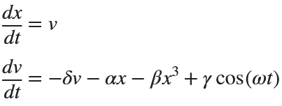
for  , the second-order equation can be transformed into the following system of first-order equations:
Exploring the Effect of γ.
% Define parameters
gamma = 0.1;
alpha = -1;
beta = 1;
delta = 0.1;
omega = 1.4;
% Define the system of equations
odeSystem = @(t, y) [y(2);
-delta*y(2) - alpha*y(1) - beta*y(1)^3 + gamma*cos(omega*t)];
% Initial conditions
y0 = [0; 0]; % x(0) = 0, v(0) = 0
% Time span
tspan = [0 200];
% Solve the system
[t, y] = ode45(odeSystem, tspan, y0);
% Plot the results
figure;
plot(t, y(:, 1));
xlabel('Time');
ylabel('x(t)');
title('Solution of the nonlinear system');
grid on;
% Plot the phase portrait
figure;
plot(y(:, 1), y(:, 2));
xlabel('x(t)');
ylabel('v(t)');
title('Phase Portrait');
grid on;
% Define the tail (e.g., last 10% of the time interval)
tail_start = floor(0.9 * length(t)); % Starting index for the tail
tail_end = length(t); % Ending index for the tail
% Plot the tail of the solution
figure;
plot(y(tail_start:tail_end, 1), y(tail_start:tail_end, 2), 'r', 'LineWidth', 1.5);
xlabel('x(t)');
ylabel('v(t)');
title('Phase Portrait - Tail of the Solution');
grid on;
% Define parameters
gamma = 0.318;
alpha = -1;
beta = 1;
delta = 0.1;
omega = 1.4;
% Define the system of equations
odeSystem = @(t, y) [y(2);
-delta*y(2) - alpha*y(1) - beta*y(1)^3 + gamma*cos(omega*t)];
% Initial conditions
y0 = [0; 0]; % x(0) = 0, v(0) = 0
% Time span
tspan = [0 800];
% Solve the system
[t, y] = ode45(odeSystem, tspan, y0);
% Plot the results
figure;
plot(t, y(:, 1));
xlabel('Time');
ylabel('x(t)');
title('Solution of the nonlinear system');
grid on;
% Plot the phase portrait
figure;
plot(y(:, 1), y(:, 2));
xlabel('x(t)');
ylabel('v(t)');
title('Phase Portrait');
grid on;
% Define the tail (e.g., last 10% of the time interval)
tail_start = floor(0.9 * length(t)); % Starting index for the tail
tail_end = length(t); % Ending index for the tail
% Plot the tail of the solution
figure;
plot(y(tail_start:tail_end, 1), y(tail_start:tail_end, 2), 'r', 'LineWidth', 1.5);
xlabel('x(t)');
ylabel('v(t)');
title('Phase Portrait - Tail of the Solution');
grid on;
% Define parameters
gamma = 0.338;
alpha = -1;
beta = 1;
delta = 0.1;
omega = 1.4;
% Define the system of equations
odeSystem = @(t, y) [y(2);
-delta*y(2) - alpha*y(1) - beta*y(1)^3 + gamma*cos(omega*t)];
% Initial conditions
y0 = [0; 0]; % x(0) = 0, v(0) = 0
% Time span with more points for better resolution
tspan = linspace(0, 200,2000); % Increase the number of points
% Solve the system
[t, y] = ode45(odeSystem, tspan, y0);
% Plot the results
figure;
plot(t, y(:, 1));
xlabel('Time');
ylabel('x(t)');
title('Solution of the nonlinear system');
grid on;
% Plot the phase portrait
figure;
plot(y(:, 1), y(:, 2));
xlabel('x(t)');
ylabel('v(t)');
title('Phase Portrait');
grid on;
% Define the tail (e.g., last 10% of the time interval)
tail_start = floor(0.9 * length(t)); % Starting index for the tail
tail_end = length(t); % Ending index for the tail
% Plot the tail of the solution
figure;
plot(y(tail_start:tail_end, 1), y(tail_start:tail_end, 2), 'r', 'LineWidth', 1.5);
xlabel('x(t)');
ylabel('v(t)');
title('Phase Portrait - Tail of the Solution');
grid on;
ax = gca;
chart = ax.Children(1);
datatip(chart,0.5581,-0.1126);
% Define parameters
gamma = 0.35;
alpha = -1;
beta = 1;
delta = 0.1;
omega = 1.4;
% Define the system of equations
odeSystem = @(t, y) [y(2);
-delta*y(2) - alpha*y(1) - beta*y(1)^3 + gamma*cos(omega*t)];
% Initial conditions
y0 = [0; 0]; % x(0) = 0, v(0) = 0
% Time span with more points for better resolution
tspan = linspace(0, 400,3000); % Increase the number of points
% Solve the system
[t, y] = ode45(odeSystem, tspan, y0);
% Plot the results
figure;
plot(t, y(:, 1));
xlabel('Time');
ylabel('x(t)');
title('Solution of the nonlinear system');
grid on;
% Plot the phase portrait
figure;
plot(y(:, 1), y(:, 2));
xlabel('x(t)');
ylabel('v(t)');
title('Phase Portrait');
grid on;
% Define the tail (e.g., last 10% of the time interval)
tail_start = floor(0.9 * length(t)); % Starting index for the tail
tail_end = length(t); % Ending index for the tail
% Plot the tail of the solution
figure;
plot(y(tail_start:tail_end, 1), y(tail_start:tail_end, 2), 'r', 'LineWidth', 1.5);
xlabel('x(t)');
ylabel('v(t)');
title('Phase Portrait - Tail of the Solution');
grid on;
Hi everyone, I am from India ..Suggest some drone for deploying code from Matlab.
Studying the attached document Duffing Equation from the University of Colorado, I noticed that there is an analysis of The Non-Chaotic Duffing Equation and all the graphs were created with Matlab. And since the code is not given I took the initiative to try to create the same graphs with the following code.
- Plotting the Potential Energy and Identifying Extrema
% Define the range of x values
x = linspace(-2, 2, 1000);
% Define the potential function V(x)
V = -x.^2 / 2 + x.^4 / 4;
% Plot the potential function
figure;
plot(x, V, 'LineWidth', 2);
hold on;
% Mark the minima at x = ±1
plot([-1, 1], [-1/4, -1/4], 'ro', 'MarkerSize', 5, 'MarkerFaceColor', 'g');
% Add LaTeX title and labels
title('Duffing Potential Energy: $$V(x) = -\frac{x^2}{2} + \frac{x^4}{4}$$', 'Interpreter', 'latex');
xlabel('$$x$$', 'Interpreter', 'latex');
ylabel('$$V(x)$$','Interpreter', 'latex');
grid on;
hold off;
- Solving and Plotting the Duffing Equation
% Define the system of ODEs for the non-chaotic Duffing equation
duffing_ode = @(t, X) [X(2);
X(1) - X(1).^3];
% Time span for the simulation
tspan = [0 10];
% Initial conditions [x(0), v(0)]
initial_conditions = [1; 1];
% Solve the ODE using ode45
[t, X] = ode45(duffing_ode, tspan, initial_conditions);
% Extract displacement (x) and velocity (v)
x = X(:, 1);
v = X(:, 2);
% Plot both x(t) and v(t) in the same figure
figure;
plot(t, x, 'b-', 'LineWidth', 2); % Plot x(t) with blue line
hold on;
plot(t, v, 'r--', 'LineWidth', 2); % Plot v(t) with red dashed line
% Add title, labels, and legend
title(' Component curve solutions to $$\ddot{x}-x+x^3=0$$','Interpreter', 'latex');
xlabel('t','Interpreter', 'latex');
ylabel('$$x(t) $$ and $$v(t) $$','Interpreter', 'latex');
legend('$$x(t)$$', ' $$v(t)$$','Interpreter', 'latex');
grid on;
hold off;
% Phase portrait with nullclines, equilibria, and vector field
figure;
hold on;
% Plot phase portrait
plot(x, v,'r', 'LineWidth', 2);
% Plot equilibrium points
plot([0 1 -1], [0 0 0], 'ro', 'MarkerSize', 5, 'MarkerFaceColor', 'g');
% Create a grid of points for the vector field
[x_vals, v_vals] = meshgrid(linspace(-2, 2, 20), linspace(-1, 1, 20));
% Compute the vector field components
dxdt = v_vals;
dvdt = x_vals - x_vals.^3;
% Plot the vector field
quiver(x_vals, v_vals, dxdt, dvdt, 'b');
% Set axis limits to [-1, 1]
xlim([-1.7 1.7]);
ylim([-1 1]);
% Labels and title
title('Phase-Plane solutions to $$\ddot{x}-x+x^3=0$$','Interpreter', 'latex');
xlabel('$$ (x)$$','Interpreter', 'latex');
ylabel('$$v(v)$$','Interpreter', 'latex');
grid on;
hold off;


