Results for
I got thoroughly nerd-sniped by this xkcd, leading me to wonder if you can use MATLAB to figure out the dice roll for any given (rational) probability. Well, obviously you can. The question is how. Answer: lots of permutation calculations and convolutions.
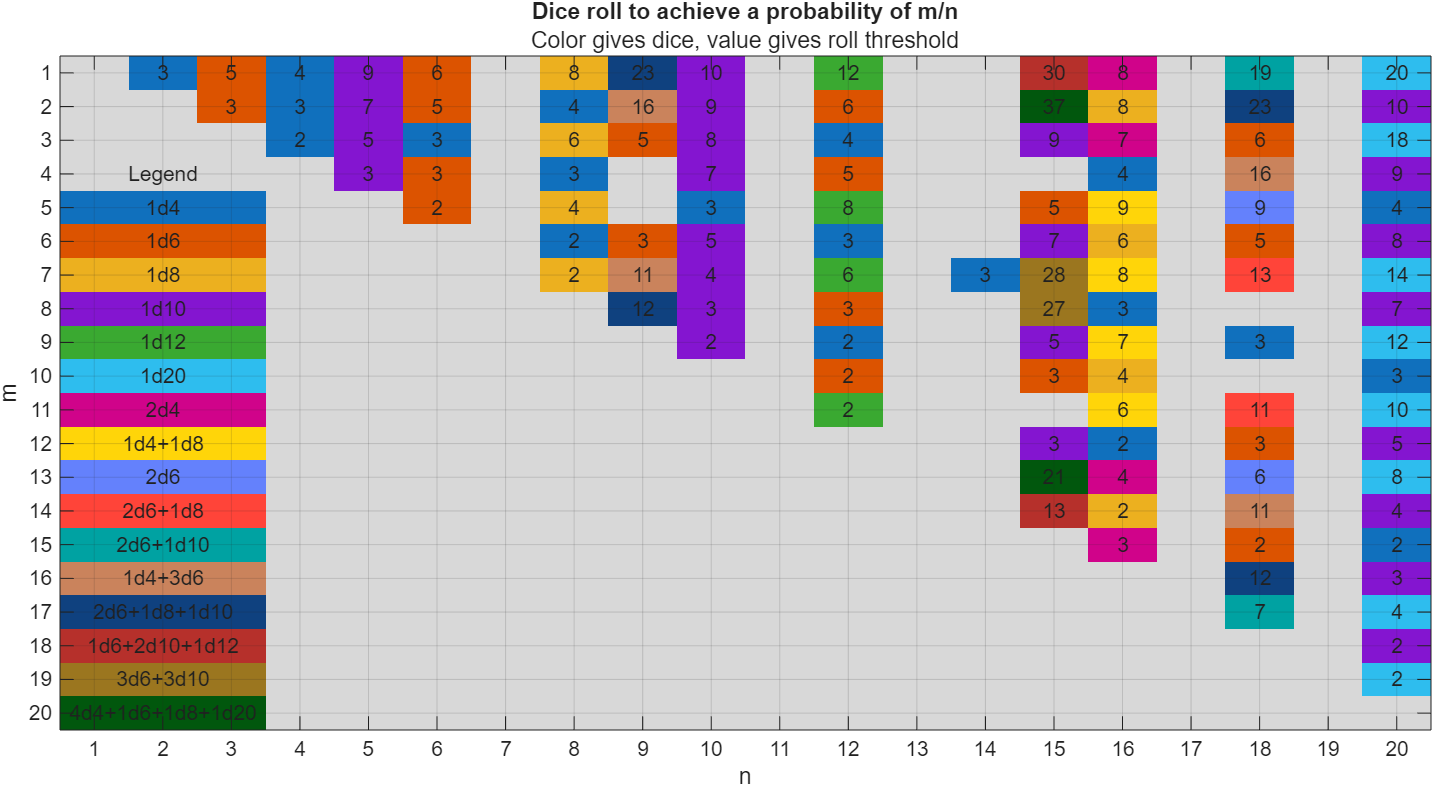
In the original xkcd, the situation described by the player has a probability of 2/9. Looking up the plot, row 2 column 9, shows that you need 16 or greater on (from the legend) 1d4+3d6, just as claimed.
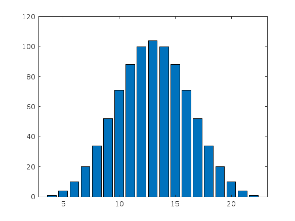
If you missed the bit about convolutions, this is a super-neat trick
[v,c] = dicedist([4 6 6 6]);
bar(v,c)
% Probability distribution of dice given by d
function [vals,counts] = dicedist(d)
% d is a vector of number of sides
n = numel(d); % number of dice
% Use convolution to count the number of ways to get each roll value
counts = 1;
for k = 1:n
counts = conv(counts,ones(1,d(k)));
end
% Possible values range from n to sum(d)
maxtot = sum(d);
vals = n:maxtot;
end
I am very pleased to share my book, with coauthors Professor Richard Davis and Associate Professor Sam Toan, titled "Chemical Engineering Analysis and Optimization Using MATLAB" published by Wiley: https://www.wiley.com/en-us/Chemical+Engineering+Analysis+and+Optimization+Using+MATLAB-p-9781394205363
Also in The MathWorks Book Program:
Chemical Engineering Analysis and Optimization Using MATLAB® introduces cutting-edge, highly in-demand skills in computer-aided design and optimization. With a focus on chemical engineering analysis, the book uses the MATLAB platform to develop reader skills in programming, modeling, and more. It provides an overview of some of the most essential tools in modern engineering design.
Chemical Engineering Analysis and Optimization Using MATLAB® readers will also find:
- Case studies for developing specific skills in MATLAB and beyond
- Examples of code both within the text and on a companion website
- End-of-chapter problems with an accompanying solutions manual for instructors
This textbook is ideal for advanced undergraduate and graduate students in chemical engineering and related disciplines, as well as professionals with backgrounds in engineering design.
Overview
Authors:
- Narayanaswamy P.R. Iyer
- Provides Simulink models for various PWM techniques used for inverters
- Presents vector and direct torque control of inverter-fed AC drives and fuzzy logic control of converter-fed AC drives
- Includes examples, case studies, source codes of models, and model projects from all the chapters.
About this book
Successful development of power electronic converters and converter-fed electric drives involves system modeling, analyzing the output voltage, current, electromagnetic torque, and machine speed, and making necessary design changes before hardware implementation. Inverters and AC Drives: Control, Modeling, and Simulation Using Simulink offers readers Simulink models for single, multi-triangle carrier, selective harmonic elimination, and space vector PWM techniques for three-phase two-level, multi-level (including modular multi-level), Z-source, Quasi Z-source, switched inductor, switched capacitor and diode assisted extended boost inverters, six-step inverter-fed permanent magnet synchronous motor (PMSM), brushless DC motor (BLDCM) and induction motor (IM) drives, vector-controlled PMSM, IM drives, direct torque-controlled inverter-fed IM drives, and fuzzy logic controlled converter-fed AC drives with several examples and case studies. Appendices in the book include source codes for all relevant models, model projects, and answers to selected model projects from all chapters.
This textbook will be a valuable resource for upper-level undergraduate and graduate students in electrical and electronics engineering, power electronics, and AC drives. It is also a hands-on reference for practicing engineers and researchers in these areas.
I want to share a new book "Introduction to Digital Control - An Integrated Approach, Springer, 2024" available through https://link.springer.com/book/10.1007/978-3-031-66830-2.
This textbook presents an integrated approach to digital (discrete-time) control systems covering analysis, design, simulation, and real-time implementation through relevant hardware and software platforms. Topics related to discrete-time control systems include z-transform, inverse z-transform, sampling and reconstruction, open- and closed-loop system characteristics, steady-state accuracy for different system types and input functions, stability analysis in z-domain-Jury’s test, bilinear transformation from z- to w-domain, stability analysis in w-domain- Routh-Hurwitz criterion, root locus techniques in z-domain, frequency domain analysis in w-domain, control system specifications in time- and frequency- domains, design of controllers – PI, PD, PID, phase-lag, phase-lead, phase-lag-lead using time- and frequency-domain specifications, state-space methods- controllability and observability, pole placement controllers, design of observers (estimators) - full-order prediction, reduced-order, and current observers, system identification, optimal control- linear quadratic regulator (LQR), linear quadratic Gaussian (LQG) estimator (Kalman filter), implementation of controllers, and laboratory experiments for validation of analysis and design techniques on real laboratory scale hardware modules. Both single-input single-output (SISO) and multi-input multi-output (MIMO) systems are covered. Software platform of MATLAB/Simlink is used for analysis, design, and simulation and hardware/software platforms of National Instruments (NI)/LabVIEW are used for implementation and validation of analysis and design of digital control systems. Demonstrating the use of an integrated approach to cover interdisciplinary topics of digital control, emphasizing theoretical background, validation through analysis, simulation, and implementation in physical laboratory experiments, the book is ideal for students of engineering and applied science across in a range of concentrations.
I am excited to share my new book "Introduction to Mechatronics - An Integrated Approach, Springer, 2023" available through https://link.springer.com/book/10.1007/978-3-031-29320-7.
This textbook presents mechatronics through an integrated approach covering instrumentation, circuits and electronics, computer-based data acquisition and analysis, analog and digital signal processing, sensors, actuators, digital logic circuits, microcontroller programming and interfacing. The use of computer programming is emphasized throughout the text, and includes MATLAB for system modeling, simulation, and analysis; LabVIEW for data acquisition and signal processing; and C++ for Arduino-based microcontroller programming and interfacing. The book provides numerous examples along with appropriate program codes, for simulation and analysis, that are discussed in detail to illustrate the concepts covered in each section. The book also includes the illustration of theoretical concepts through the virtual simulation platform Tinkercad to provide students virtual lab experience.
I had originally planned on publishing my book via a traditional publisher, but am now reconsidering whether to use Amazon.com. I use Matlab and Latex in my book. It appears that it is not possible to publish is with Amazon due to this. Advice? Thanks. Kevin Passino
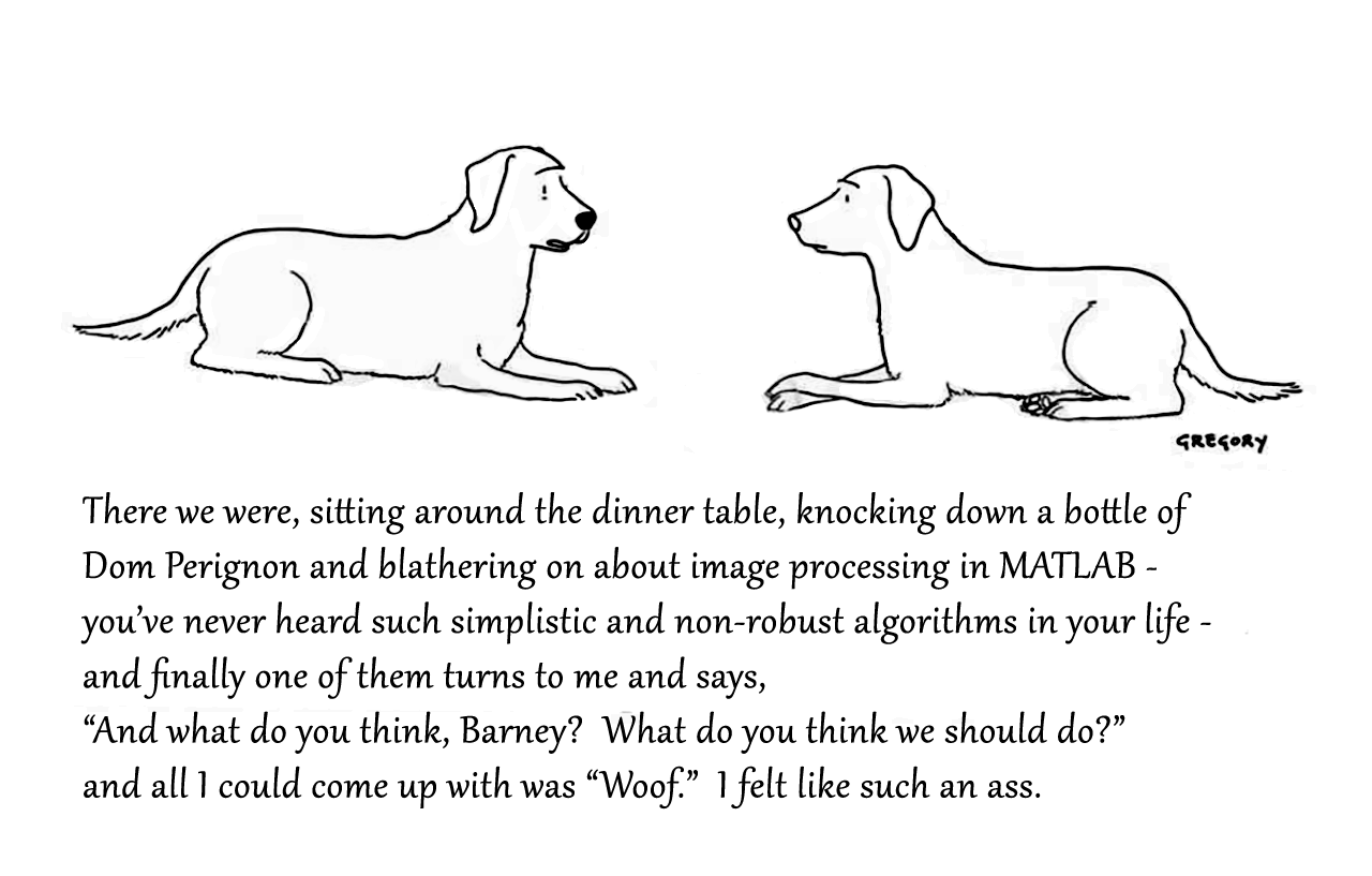
Attaching the Photoshop file if you want to modify the caption.

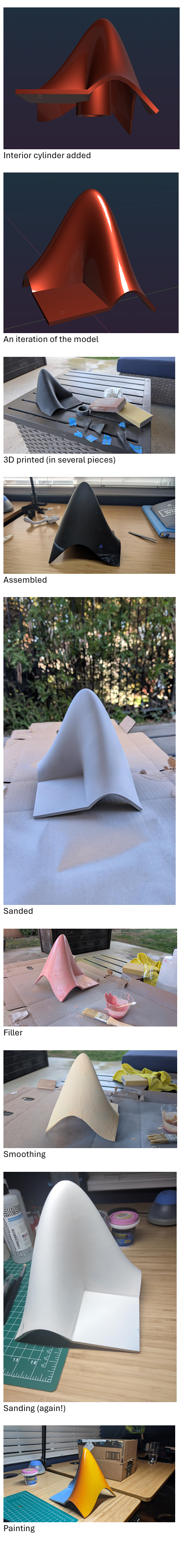
What better way to add a little holiday magic than the L-shaped membrane atop your evergreen? My colleagues output the shape and then added some thickness and an interior cylinder in Blender. Then, the shape was exported to STL and 3D printed (in several pieces). Then glued, sanded, primed, sanded again and painted. If you like, the STL file is attached. Thank you to https://blogs.mathworks.com/community/2013/06/20/paul-prints-the-l-shaped-membrane/ and a tip of the hat to MATLAB Ornament. Happy Holidays!


I am very excited to share my new book "Data-driven method for dynamic systems" available through SIAM publishing: https://epubs.siam.org/doi/10.1137/1.9781611978162
This book brings together modern computational tools to provide an accurate understanding of dynamic data. The techniques build on pencil-and-paper mathematical techniques that go back decades and sometimes even centuries. The result is an introduction to state-of-the-art methods that complement, rather than replace, traditional analysis of time-dependent systems. One can find methods in this book that are not found in other books, as well as methods developed exclusively for the book itself. I also provide an example-driven exploration that is (hopefully) appealing to graduate students and researchers who are new to the subject.
Each and every example for the book can be reproduced using the code at this repo: https://github.com/jbramburger/DataDrivenDynSyst
Hope you like it!
Christmas season is underway at my house:

(Sorry - the ornament is not available at the MathWorks Merch Shop -- I made it with a 3-D printer.)
My favorite image processing book is The Image Processing Handbook by John Russ. It shows a wide variety of examples of algorithms from a wide variety of image sources and techniques. It's light on math so it's easy to read. You can find both hardcover and eBooks on Amazon.com Image Processing Handbook
There is also a Book by Steve Eddins, former leader of the image processing team at Mathworks. Has MATLAB code with it. Digital Image Processing Using MATLAB
You might also want to look at the free online book http://szeliski.org/Book/
I know we have all been in that all-too-common situation of needing to inefficiently identify prime numbers using only a regular expression... and now Matt Parker from Standup Maths helpfully released a YouTube video entitled "How on Earth does ^.?$|^(..+?)\1+$ produce primes?" in which he explains a simple regular expression (aka Halloween incantation) which matches composite numbers:
Here is my first attempt using MATLAB and Matt Parker's example values:
fnh = @(n) isempty(regexp(repelem('*',n),'^.?$|^(..+?)\1+$','emptymatch'));
fnh(13)
fnh(15)
fnh(101)
fnh(1000)
Feel free to try/modify the incantation yourself. Happy Halloween!
Hello! The MathWorks Book Program is thrilled to welcome you to our discussion channel dedicated to books on MATLAB and Simulink. Here, you can:
- Promote Your Books: Are you an author of a book on MATLAB or Simulink? Feel free to share your work with our community. We’re eager to learn about your insights and contributions to the field.
- Request Recommendations: Looking for a book on a specific topic? Whether you're diving into advanced simulations or just starting with MATLAB, our community is here to help you find the perfect read.
- Ask Questions: Curious about the MathWorks Book Program, or need guidance on finding resources? Post your questions and let our knowledgeable community assist you.
We’re excited to see the discussions and exchanges that will unfold here. Whether you're an expert or beginner, there's a place for you in our community. Let's embark on this journey together!
In case you haven't come across it yet, @Gareth created a Jokes toolbox to get MATLAB to tell you a joke.
Hi All,
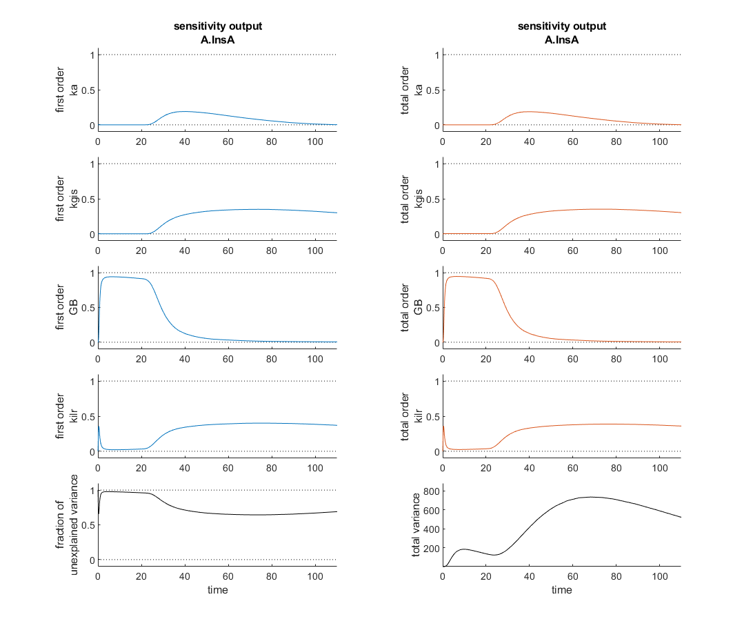
I'm currently verifying a global sensitivity analysis done in SimBiology and I'm a touch confused. This analysis was run with every parameter and compartment volume in the model. To my understanding the fraction of unexplained variance is 1 - the sum of the first order variances, therefore if the model dynamics are dominated by interparameter effects you might see a higher fraction of unexplained variance. In this analysis however, as the attached figure shows (with input at t=20 minutes), the most sensitive four parameters seem to sum, in first order sensitivities to roughly one at each time point and the total order sensitivies appear nearly identical. So how is the fraction of unexplained variance near one?
Thank you for your help!
Imagine that the earth is a perfect sphere with a radius of 6371000 meters and there is a rope tightly wrapped around the equator. With one line of MATLAB code determine how much the rope will be lifted above the surface if you cut it and insert a 1 meter segment of rope into it (and then expand the whole rope back into a circle again, of course).
Hi to everyone!
To simplify the explanation and the problem, I simulated the kinetics of an irreversible first-order reaction, A -> B. I implemented it in two independent compartments, R and P. I simulated the effect of a dilution in R by doubling at t= 0,1 the R volume. I programmed in P that, at t = 0.1, the instantaneous concentration of A and B would be reduced by half. I am sending an attach with the implementation of these simulations in the Simbiology interface.
When the simulations of the two compartments are plotted, it can be seen that the responses are not equal. That is, from t = 0.1 s, the reaction follow an exponential function in R with half of the initial amplitude and half of the initial value of k1. That is, the relaxation time is doubled. Meanwhile, in P, from t = 0.1, the reaction follows exponential kinetics with half the amplitude value but maintaining the initial value of k = 10. Without a doubt, the correct simulation is the latter (compartment P) where only the effect is observed in the amplitude and not in the relaxation time. Could you tell me what the error is that makes these kinetics that should be equal not be?
Thank you in advance!
Luis B.
Hi All,
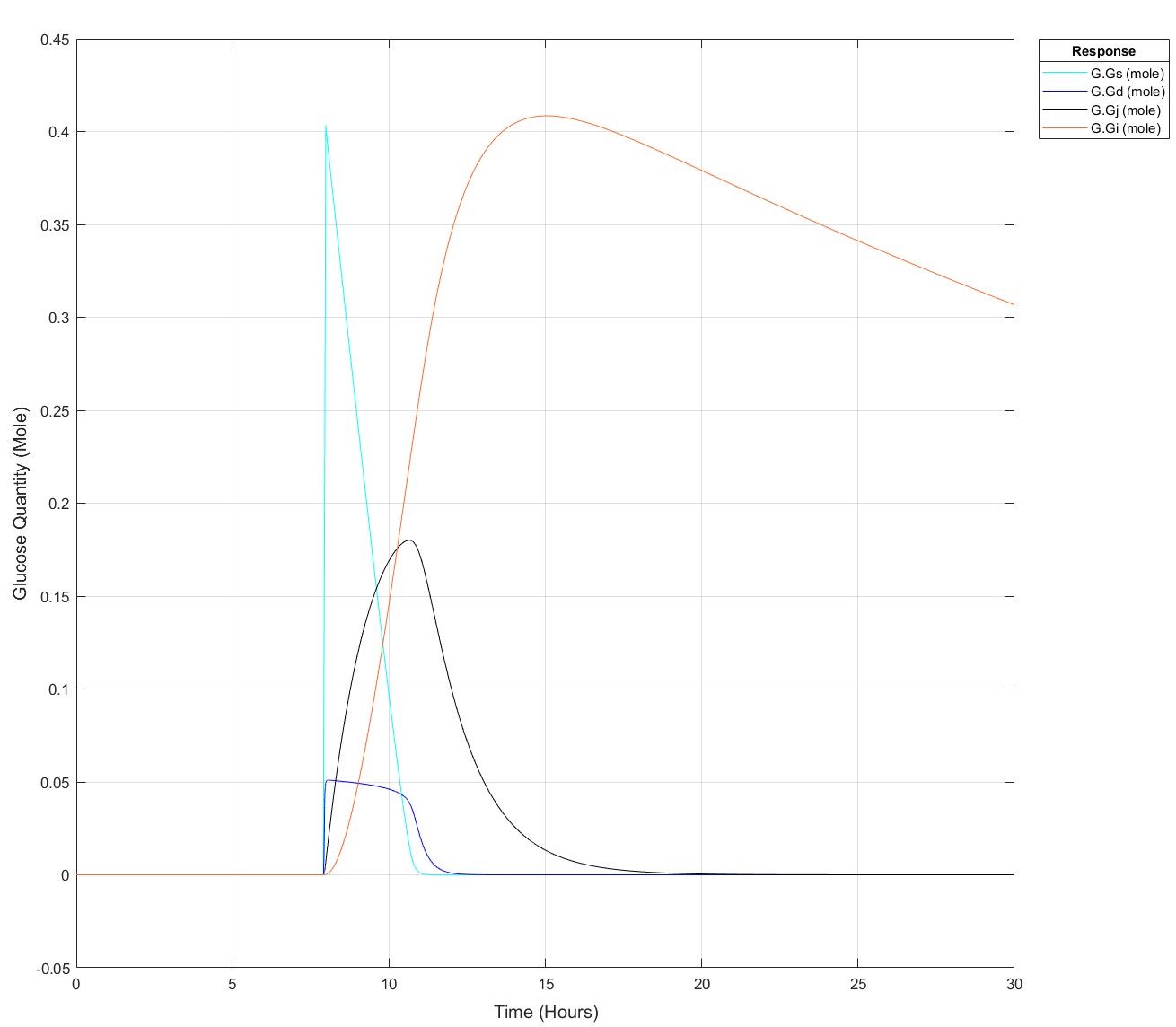
I've been producing a QSP model of glucose homeostasis for a while now for my PhD project, recently I've been able to expand it to larger time series, i.e. 2 days of data rather than a singular injection or a singular meal. My problem is as follows: If I put 75g of glucose into my stomach glucose species any later than (exactly) 8.5 hours I get an integration tolerance error. Curiosly, I can put 25g of glucose in at any time up to 15.9 hours, then any later an error. I have disabled all connections to my glucose absorption chain, i.e. stomach -> duodenum -> jenenum -> ileum -> removal, to isolate the cause of this. I had initially thought it may be because I mechanistically model liver glycogen and that does deplete over time, but I've tested enough to show that that does nothing. My next test is to isolate the glucose absorption chain into a seperate model and see if the issue persists but I'm completely baffled!
These are the equations, to my eye there's no reason why there would be such a sharp glucose quantity/time dependence, they all begin at a value of 0:
d(Gs)/dt = -(kw*(1-Gd^14/(Igd^14+Gd^14))*Gs) #Stomach glucose
d(Gd)/dt = (kw*(1-Gd^14/(Igd^14+Gd^14))*Gs) - (kdj*Gd) #Duodenal Glucose
d(Gj)/dt = (kdj*Gd) - (kji*Gj) #Jejunal Glucose
d(Gi)/dt = (kji*Gj) - (kic*Gi) #Ileal Glucose
(The sigmoidicity of gastric emptying slowing term (^14) was parameterised off of paracetamol absorption data and appears to be correct!)
Thank you for your help, best regards,
Dan
Pre-Edit: I changed the run time to 30 hours and now I can't use the 75g input any later than 7.9 hours not 8.5 hours anymore!
Edit: This is how it appears at all times prior to it failing for 75g: