Applying Machine Learning Techniques to Classify Musical Instrument Loudspeakers

Celestion loudspeakers have powered the performances of many noted guitar and bass players, including legends such as Jimi Hendrix. Deciding whether a loudspeaker is good enough for professional musicians is a lengthy and painstaking process. Each speaker has its own unique sound based on a combination of sonic characteristics, such as midrange character and brightness. Evaluating a musical instrument loudspeaker involves subjective judgement about whether it generates a “good” sound. Only engineers with years of experience can reliably make that decision, and then only after repeated listening to a single loudspeaker and comparing the sounds it produces with those produced by a reference speaker.

As a member of the Celestion R&D team, I recently tackled the problem of automating this manual process, to free up time from listening tests that are regularly repeated. Using MATLAB^®, Statistics and Machine Learning Toolbox™, and Signal Processing Toolbox™, I developed an application that uses machine learning algorithms to classify one loudspeaker model as either good or bad. The application can judge a speaker accurately and consistently in seconds, and its results are both consistent and repeatable. The repeated blind listening tests needed for a confident judgement would take far longer, and would require an extra pair of hands.

Streamlining the Manual Classification Process with MATLAB

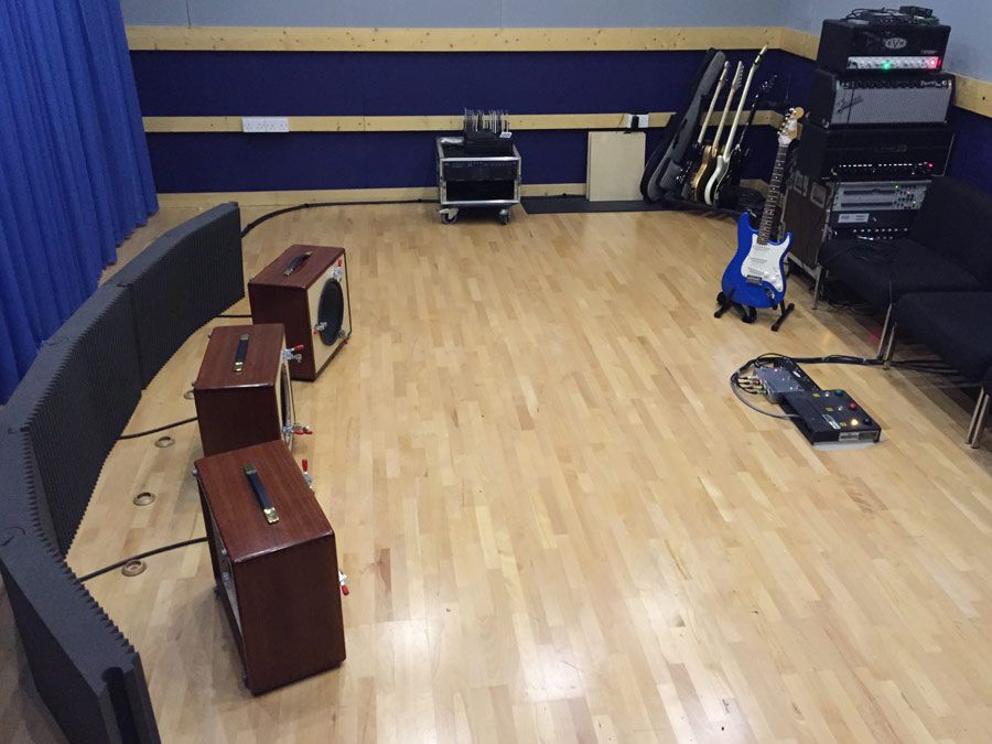
To classify a single speaker manually, an engineer listens to the sound it produces as a guitar is played through it and compares that to the sound produced by a known good reference speaker with the same guitar and amp. This work is done in our specially designed listening room (Figure 1). The engineer is not looking for a speaker that sounds exactly like the reference but for one that sounds as good as the reference and is within a subjectively determined sonic range. For a confident classification, a speaker has to receive the same rating at least nine times in ten independent listening tests.

With most bad speakers, the engineer can switch between the two speakers and hear the difference in sound as certain chords decay. We normally do this by switching between speakers with our bespoke switching setup, shown in Figure 1. However, the speakers must be physically swapped after two listening tests. With large numbers of speakers, and each individual speaker being listened to ten times, this physical process becomes labor-intensive.

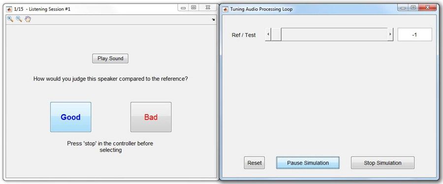
To streamline this part of the process, I developed a MATLAB application that trained listeners can use to switch between the reference and test speakers in real time. I used Audio Toolbox™ to stream real-time audio directly from MATLAB, created the main UI for playing and selection, and borrowed an example from the documentation to create a second UI for switching tracks interactively during playback (Figure 2).

Using this application, engineers can classify a large batch of speakers in one hour instead of eight, and without the extra person previously required to help change speakers. Human input is only required for training purposes; the final machine learning program is based purely on electroacoustic measurements, and produces results equivalent to repeated listening tests.

Machine learning was the right tool to find the most suitable distinction between groups of measurements on which to base a test. A key benefit is that a machine learning algorithm learns and adapts the boundary if more information is presented later. This means that the program can be updated to adapt to changing components or tastes.

Having established that machine learning was the tool for the job, I had to begin building my skills almost from scratch.

Learning Machine Learning

To get started, I enrolled in a massive open online course (MOOC) taught by Andrew Ng of Stanford University. The course provides an introduction to machine learning techniques and concepts, including linear regression, logistic regression, neural networks, and support vector machines (SVMs). I completed course assignments by manually coding machine learning algorithms in MATLAB.

Those exercises gave me an appreciation of the basics, allowing me to apply different methods manually as I learned them in the course. However, I saw a significant improvement in results when I got Statistics and Machine Learning Toolbox. Once I began using the toolbox, I found that I could accomplish in a few clicks what took me hours or days to program and debug manually. It was simple to build and compare many complex models, each of which would have taken days, if not weeks of work to code manually.

Creating a Labeled Dataset

To train a machine learning classifier, I first needed to build a labeled dataset. For this project, the dataset was a large number of loudspeaker measurements, each correctly labeled as good or bad based on listening tests.

Having gathered 60 speakers for the preliminary investigation, I could have run traditional listening tests using each speaker, but that would have been a long and costly process. Instead, I used offline recordings of each loudspeaker together with the app that I had developed. This allowed for instant changeover of wav files rather than manual changeover of speakers. Putting that app in the hands of expert listeners allowed me to build a labeled dataset in a fraction of the time that it would have taken using a traditional approach.

Selecting Features to Train Machine Learning Algorithms

To train the machine learning classifier, I not only needed to label each speaker as “good” or “bad,” I also needed to preprocess the raw measurements to extract representative numerical inputs, or features, that the classifiers could work with. I developed and examined more than 50 features over several months. These included energy features, such as the energy center; spectral features, such as high-frequency roll-off and brightness; and psychoacoustic features, such as sharpness.

Psychoacoustics features relate to how humans perceive sound, and as a result, correlate strongly to the separation seen between good and bad groups of speakers.

Unlike frequency response, which can be measured directly, psychoacoustic features must be computed from measured values. To compute psychoacoustic values, I used MATLAB, Signal Processing Toolbox, and DSP System Toolbox™ to implement established formulas for psychoacoustics from a range of textbooks. I applied functions for smoothing, convolution, peak finding, and computing Welch’s power spectral density (PSD) estimates, among others.

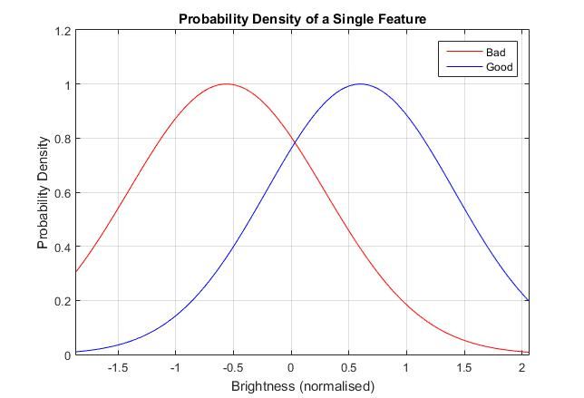
I selected a subset of 27 features to serve as inputs to the machine learning algorithm. For a feature to be included it had to correlate well with a speaker’s good or bad grouping. No individual feature was sufficient by itself.  For example, brightness has one of the best correlations with the good/bad separation, but a plot of the probability density function reveals considerable overlap for good and bad speakers (Figure 3).

The result could be predicted, but with very limited certainty. Our idea was that in combining many results, the degree of certainty would increase. Rather than a linear ‘hurdle’ type approach, machine learning would enable us to consider the values of all features at once and then calculate the overall probability of a good result.

Developing and coding features for comparison was the most time-consuming part, and provided some great new tools for analysis. Once these had been developed it was time to assess which statistical method would work best.

Applying Logistic Regression to Multiple Features

Starting with the simplest method, logistic regression is a well-known binary classifier that works by finding an optimal decision boundary between features to separate one class from the other. For a single feature, the decision boundary is represented by a single value. One side of the boundary is defined as good, the other side as bad. I had already seen that no single feature was sufficient to make an accurate classification, so I began applying linear regression with multiple features. When two features are considered, the decision boundary is a line. With three features, it is a planar (Figure 4).

I performed linear logistic regression with all 27 features, achieving a classification accuracy of around 80-85%. There are many different methods available for logistic regression. I used the Classification Learner app from Statistics and Machine Learning Toolbox to quickly experiment with different types. Even when using just a few features, the plots clearly showed that nonlinear regression with quadratic and higher-order boundaries would do a better job of separating the measurements. Exploring this approach in MATLAB, I improved performance relative to a linear boundary, increasing it to 90%.

Improving Classification Performance with Support Vector Machines

SVM classifiers are often more efficient and easier to optimize than logistic regression classifiers.

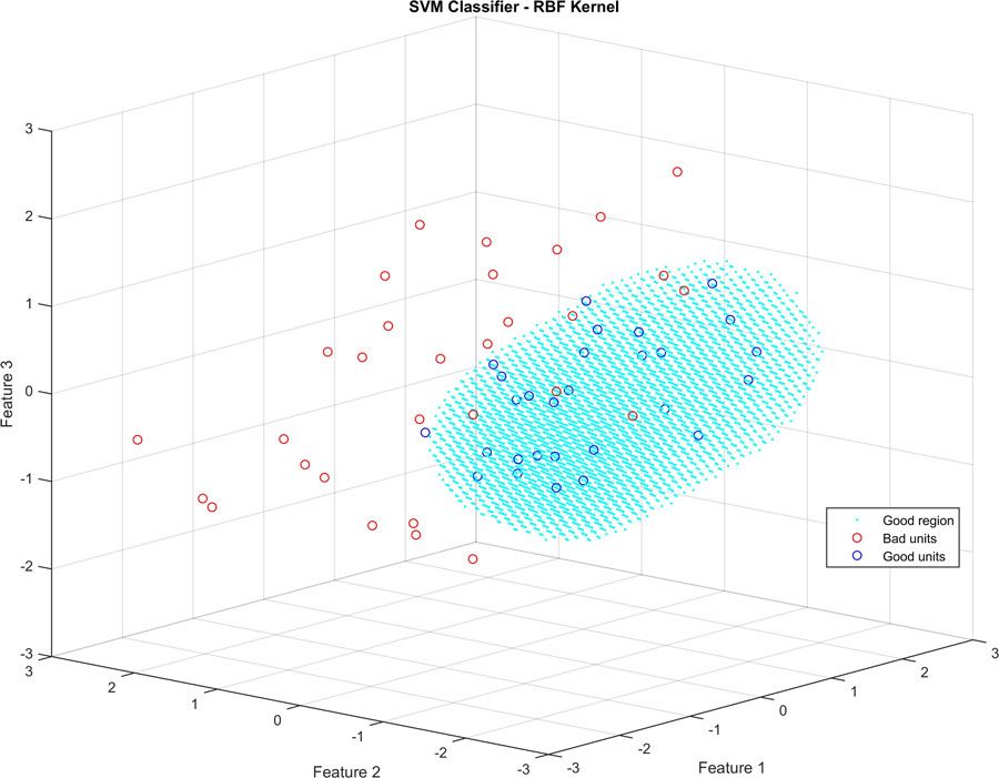
To train an SVM model I again used the Classification Learner app from Statistics and Machine Learning Toolbox. I simply specified the features I wanted to use, selected the radial basis function (RBF) kernel, and with a single click started the training. Training on the same data I had used for linear logistic regression, the SVM model had a classification accuracy of around 91%.

The plot shown in Figure 5 was created using the same features and data as those in Figure 3, but instead of being separated from bad units by a planar boundary, good units are now grouped within the volume highlighted in blue.

I also trained and predicted using artificial neural networks (ANNs) and Neural Network Toolbox™, but typically found that prediction accuracy wasn’t improved relative to SVM. This could well be due to the size of the dataset used and number of features; it’s possible that ANNs could improve results for larger datasets.

Fine-Tuning with Regularization, Ensemble Methods, and Cascade Architectures

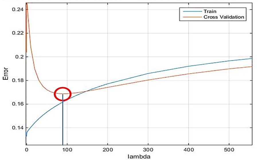
When using more than two dozen features to train a model, one risks creating an overly complex classifier that fits the training data very well but performs poorly on similar but not identical measurements. To avoid this situation I used regularization, employing a separate cross-validation dataset to ensure that the model would translate well to other datasets. By adjusting the regularization parameter lambda, I reduced the error on the cross-validation set―at the expense of a somewhat higher error on the training set. I used Optimization Toolbox™ to find an optimal value for lambda and minimize the error on both sets (Figure 6).

To further improve classification performance, I experimented with ensemble methods, again using the Classification Learner app in Statistics and Machine Learning toolbox. Ensemble methods combine several reasonably-performing classifiers into one high-performing classifier. Ensemble methods improved the performance of the model to around 92%.

Cascade architectures were originally developed to reduce computation costs when many features are used. Computational performance was not a concern for me, but the cascade architecture concept proved useful because it identified outliers in my dataset. I labeled the incorrectly classified units as anomalies and removed them, then retrained the classifier using the remaining units. I repeated this process twice to filter out the borderline units in a cascade process. This step increased the performance of the final algorithm to about 93%. This gave us a very repeatable test, saving many engineer hours and reducing the need for tedious repeated listening to a single model.

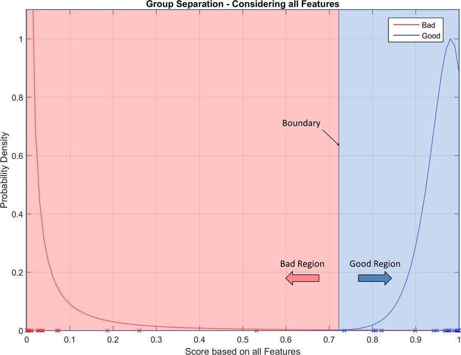
Figure 7 illustrates the greatly improved performance of the final machine learning algorithm, relative to any single feature alone¹.

These results are based on finding the optimum separation. In practice, the boundary can be adjusted to suit the task, shifting it towards the good or bad units. This makes the program flexible, allowing it to be tuned for a specific task, and giving errors of less than 0.1% for the group of highest importance. The practice of minimizing the number of incorrectly classified good units (maximum precision) or minimizing the number of incorrectly classified bad units (maximum recall) allows the algorithm to be tailored to the application.

Lessons Learned

In creating this application, I learned three lessons that will serve me well as my group expands its use of machine learning. The first is that there is value in applying simpler algorithms such as linear logistic regression, even if they end up performing poorly compared to SVM, neural networks, or ensemble methods. With more advanced machine learning techniques, it was difficult to break down and interpret the results. In this respect, I learned more about ideal performance from the simpler algorithms.

The second lesson is that with a long and open-ended process like feature extraction, having access to readily available signal processing functions is virtually a necessity—on this project it enabled me to experiment with a number of feature options in a relatively short time.

The third lesson is that no single machine learning technique works well with all datasets. The performance of each classifier algorithm depends on the size of the dataset, the type of data it contains, how many features are included, and so on. I found it impossible to predict which algorithms would work best from reading about them in textbooks. I had to just try them. If I had coded them manually, it would have taken me years. With MATLAB and Statistics and Machine Learning Toolbox, once I had data ready I could try out 10 or 20 different classifier methods in minutes.

¹These results are based on preliminary data and are soon to be superseded by incorporating results from an additional hundred units.