Engaging Students in Hands-On System Identification and Controller Design at University of Arizona
By Eniko T. Enikov, University of Arizona
“This hands-on work complements the lecture portion of our courses with active, sensory learning that gets students excited about control design and system identification.”
In their senior year, approximately 130 mechanical and aerospace engineering students at the University of Arizona complete their required training in control system design. Recently, our department implemented a dedicated laboratory course on dynamics and controls to supplement the traditional lecture-based courses in system identification and controls. The purpose of the laboratory is to provide engaging and meaningful design activities for a large cohort of students with relatively limited prior knowledge of control theory. Developing such a course has been challenging, as it requires balancing low operating costs while providing each student with sufficient time for hands-on experimentation and analysis.
To address this need, we have recently developed a portable wireless laboratory module based on MATLAB®, Simulink®, Arduino® Nano 33 IoT, and a twin-propeller balancing beam (the Balancing Bi-Copter) (Figure 1). Students take the device home or work independently in the library to conduct experiments and complete assignments. This hands-on work complements the lecture portion of our courses with active, sensory learning that gets students excited about control design and system identification.

Figure 1. The Balancing Bi-Copter. (Image credit: The University of Arizona Department of Aerospace & Mechanical Engineering/Rachel Spitz)
Teaching Control Design Basics
The bi-copter is introduced in the second half of the semester; in the first half, students learn basic control theory and how to model simple electromechanical systems such as DC motors and spring-mass systems. They also develop system identification skills and model parameter extraction from experimental data, including initially static systems and subsequently dynamic systems. In the lectures, I use MATLAB and Simulink to illustrate new concepts. For example, when I cover the analysis of block diagrams and building dynamic models, I use MATLAB and Simulink to create a visual simulation. One of the lab’s new features is the inclusion of system identification topics, beginning with simple experiments that use linear regression to determine the coefficients of a static model, and advancing to nonlinear regression techniques that simultaneously estimate parameters such as gain, natural frequency, and damping coefficient from input-output data. The lab module has a short introductory lecture, where I show students a step-by-step manual derivation of the formulas for extracting the parameters. This is followed by an illustration of functions in System Identification Toolbox™, which enables students to perform model parameter extraction more efficiently.
When they begin the laboratory experimentation, most students are familiar with basic MATLAB commands, having used them in their numerical methods course. Few, however, have any experience with Simulink or control and system identification tools. To help students learn Simulink, I incrementally build Simulink models in class and provide templates with empty blocks, which students modify to develop a complete model. A more comprehensive self-paced Simulink Onramp that students can complete online is also available.
Experimenting with the Bi-Copter
Once the students have become proficient in using Simulink and control and system identification tools, they start experimenting with the bi-copter in the second half of the semester. The goal of the activity is to develop a linear model of the plant, identify its parameters, and design a closed-loop controller that balances the beam at a desired angle. If an external disturbance is applied to the beam, the control system must return it to its correct position within two seconds.
The system identification and control design experiments with the bi-copter are available in this GitHub® repo. MATLAB live scripts, along with Simulink models, are used to conduct individual experiments covering open-loop testing, model identification, controller design, and closed-loop testing to maintain the bi-copter at the desired reference angles. In the first experiment, students send excitation signals to the bi-copter using a random binary sequence (RBS) generated by the idinput() command. The resulting bi-copter response (Figure 2) is then used to identify different black-box models such as linear ARX, transfer function, and state-space models.

Figure 2. Input-output test data.
Students then use iddata(), arx(), n4sid(), compare(), and resid() commands to identify and analyze different models of the plant. Typically, fifth- or sixth-order models provide a good fit, but even under-parameterized third-order models can be sufficient for designing closed-loop controllers, provided they adequately capture the essential dynamics of the bi-copter.
For the second assignment, students use the identified model to design PID or state-space–based servo controllers. The PID controller and its tuning methods (Zigler-Nichols) are introduced in the classical controls course. In the lab, students utilize the pidtune() command to arrive at a suitable controller. For the second method, students add an integrator to the controller and design an observer controller, which places the closed-loop poles according to the LQR (linear-quadratic regulator) theory for a single-input, single-output (SISO) system. In the associated preparatory lecture, I present the tradeoff between penalizing the input and output. For a SISO system, this is equivalent to changing a single parameter that regulates the control effort versus the speed of the response. Typically, students design two controllers—one with aggressive characteristics for a fast response and another with more conservative tuning that yields slower responses but requires less control effort.
The Bi-Copter Setup
The bi-copter uses two propellers driven by PWM signals generated by the Arduino Nano 33 IoT microcontroller board. The onboard accelerometer records the gravitational acceleration in order to compute the tilt angle of the beam. Figure 3 shows a schematic of the signal flow and the main components of the system. The bi-copter is powered by two lithium-ion batteries housed within the balancing beam, enabling wireless communication between the Arduino Nano IoT and a PC running MATLAB and Simulink. The GitHub repo contains hardware setup instructions, including the required MATLAB and Simulink hardware support packages for Arduino.

Figure 3. Diagram of the bi-copter showing the signal flow.
Open-loop and closed-loop Simulink models are used to carry out experiments in real time. Depending on the desired test, students automatically generate code from the corresponding Simulink model and deploy it to the Arduino Nano IoT board while it is connected to the PC via USB. After deployment, the bi-copter can be operated remotely over a wireless network. During the experiments, the deployed code waits for a cue (input data) from the PC to execute an open-loop or closed-loop test. Upon completion of the run, the experiment results are directly available in the live script.
The complete device can be built for less than $100 using a 3D-printed stand/holder and commercially available components from Amazon. A complete list of materials and 3D CAD files are available in the project GitHub repository.
The open-loop (Figure 4a) and closed-loop models (Figure 4b) have the option to adjust the baseline power to the propellers (zero-level signal). Furthermore, it is possible to balance the thrust of the left and right propellers by modifying the offset level. The motor direction can be specified independently for each motor. Finally, a running average finite impulse response (FIR) filter is used to reduce the noise level due to propeller vibration.
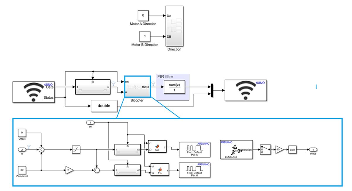
Figure 4a. Simulink model of the open-loop system.

Figure 4b. Simulink model of the closed-loop system with the PID controller.
Prior to running, each controller is compiled and deployed to the Arduino Nano 33 IoT board using a USB serial link.
Examples of input-output test data over a 20-second period are shown in Figure 2. The output signal represents the roll angle in radians, while the input signal represents PWM values on a 0–255 scale. Zero input for signal u means that both motors operate at equal power determined by the zero-level parameter. A positive input of u implies that motor A will operate at [zero-level] +u, while motor B will operate at [zero-level] –u.
Based on what they have learned about DC motors and dynamics, students develop a linear model indicating a possible fourth-order model, considering two motors working in unison (Figure 5). If the motors are modeled individually, the order would increase to five. Including additional effects, such as the inertia and air flow (added mass effect), further raises the order to six. Therefore, students anticipate that a model order in the range of four to six should be adequate.

Figure 5. A possible linear model of the bi-copter.
Analyzing the Open-Loop Response
Upon completion of the open-loop test, students proceed to system identification. Prepared with some understanding of the anticipated order, they fit different model structures of fourth, fifth, and sixth orders. Examples of continuous transfer function, ARMAX, and state-space models are shown in Figure 6 along with their comparison to the experimental data.

Figure 6. Testing open-loop models of the fourth order.
During this task, most students are perplexed by the varying results of the system identification step based on the parameters of the input test sequence. The most important parameters they test are the amplitude and frequency content of the excitation. Upon several iterations, they arrive at the conclusion that the frequency bandwidth should match the frequency of the tested poles, and the amplitude should be as high as possible within the linear limits of the response.
Model quality is examined using residual analysis implemented as the resid() command. Figure 7 shows a comparison of fourth-order ARMAX and state-space models. The ARMAX appears to have less correlated residual error, suggesting a better modeling of the underlying process.

Figure 7. Residual analysis of the identified models.
PID Controller Tuning
Upon completion of the system identification, the students proceed to design a controller. All of them are familiar with the use of PID controllers, which is the default design method. Students start with an initial guess of a PID controller:
C0 = pid(1,1,1,'Ts',ts,'IFormula','BackwardEuler','DFormula','BackwardEuler');
This controller is then used in the PID Tuner live task. Using the sliders, students adjust the grain crossover frequency and the desired phase margin and then evaluate the predicted response (Figure 8). Some students who have also completed our elective modern control course use the state-space design method as well.

Figure 8. PID tuning using a live task.
Closed-Loop Testing
Upon completion of the controller design, students test their closed-loop controller. The identified transfer function also allows them to predict the closed-loop response. Upon executing the test, the live script generates a comparison between the reference signal, the predicted response, and the measured response (Figure 9).

Figure 9. Closed-loop response of the PID-controlled bi-copter.
A more advanced controller using higher order models and the state-space design method based on LQR theory produces even more accurate tracking results (Figure 10).

Figure 10. State-space–based controller using LQR theory.
The bi-copter is also well-suited for teaching other advanced control methods such as model predictive control (MPC). The video “System Identification and MPC Design Using a Low-Cost Bi-Copter Hardware” (see the “Learn More” section at the end of this article) shows the design and deployment of an MPC controller using a data-driven prediction model for bi-copter control.
Student Feedback
Student responses to the course and the hands-on assignments have been very positive. In a course evaluation survey, we inquired about the students’ attitudes toward the hands-on experiments, the usefulness of the completed tasks, and the likelihood that the students will utilize the acquired skills in other contexts. A total of six statements were evaluated by 18 participants (Figure 11). In most categories, the project appears highly impactful, with students gaining confidence in designing controllers. It appears that the primary gains were from the hands-on components as opposed to lecturing, which is typical for undergraduate courses.
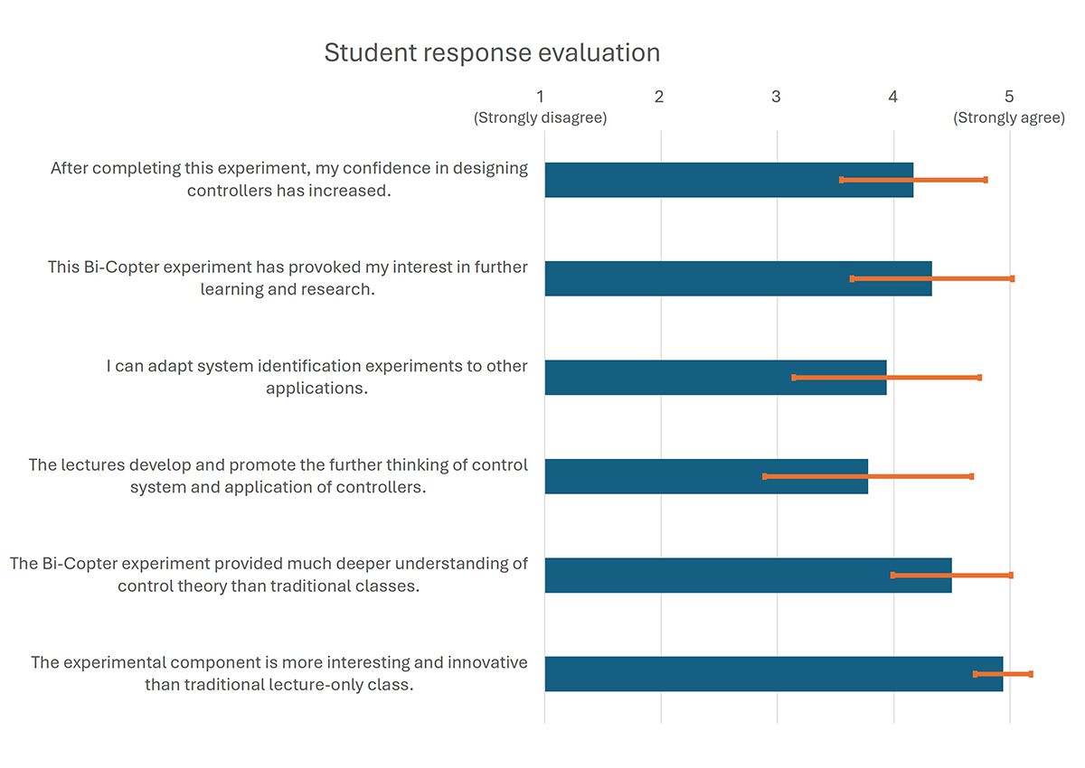
Figure 11. Student survey results (orange bars indicate standard deviation).
Informal discussions with other instructors suggest that it is very convenient to utilize a direct wireless link to the Simulink environment and MATLAB. The low cost and access to commercially assembled subcomponents make the system easy to implement at any institution. For more information, visit our GitHub page.
Published 2025 - 91891v00