margin
Gain margin, phase margin, and crossover frequencies
Syntax
Description
Margin Plots
margin( plots the Bode response
of sys)sys on the screen and indicates the gain and phase
margins on the plot. Gain margins are expressed in dB on the plot.
Solid vertical lines mark the gain margin and phase margin. The dashed
vertical lines indicate the locations of Wcp, the frequency
where the phase margin is measured, and Wcg, the frequency
where the gain margin is measured. The plot title includes the magnitude and
location of the gain and phase margin.
Gm and Pm of a system indicate the
relative stability of the closed-loop system formed by applying unit negative
feedback to sys, as shown in the following figure.
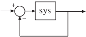
Gm is the amount of gain variance required to make the loop
gain unity at the frequency Wcg where the phase angle is
–180° (modulo 360°). In other words, the gain margin is 1/g
if g is the gain at the –180° phase frequency. Similarly, the
phase margin is the difference between the phase of the response and –180° when
the loop gain is 1.0. The frequency Wcp at which the
magnitude is 1.0 is called the unity-gain frequency or
gain crossover frequency. When sys
has more than one crossover, margin indicates the
frequencies with gain margin closest to 0 dB and phase margin closest to
0°.
Usually, gain margins of 3 or more combined with phase margins between 30°
and 60° result in reasonable tradeoffs between bandwidth and stability. However,
in some multivariable systems, stability can be lost at a different frequency
for much smaller gain and phase variations. For such systems, the notion of
disk margins provides more reliable estimates of the
true gain and phase margins. For more information on disk margins, see diskmargin (Robust Control Toolbox).
Margin Values
[
returns the gain margin Gm,Pm,Wcg,Wcp] = margin(sys)Gm in absolute units, the phase
margin Pm, and the corresponding frequencies
Wcg and Wcp, of
sys. Wcg is the frequency where
the gain margin is measured, which is a –180° phase crossing frequency.
Wcp is the frequency where the phase margin is
measured, which is a 0-dB gain crossing frequency. These frequencies are
expressed in radians/TimeUnit, where
TimeUnit is the unit specified in the
TimeUnit property of sys. When
sys has several crossovers, margin
returns the smallest gain and phase margins and corresponding
frequencies.
margin returns a warning if your system is not internally
stable, that is, if your system is not closed-loop stable or contains pole-zero
cancellations outside of the open left-half plane.
Examples
For this example, create a continuous transfer function.
sys = tf(1,[1 2 1 0])
sys =

         1
  ---------------
  s^3 + 2 s^2 + s

Continuous-time transfer function.
Model Properties
Display the gain and phase margins graphically.
margin(sys)
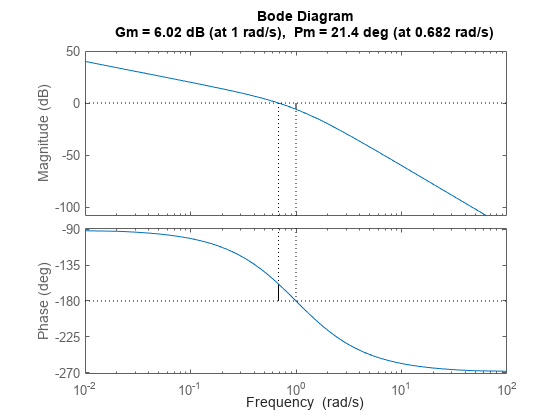
The gain margin (6.02 dB) and phase margin (21.4 deg), displayed in the title, are marked with solid vertical lines. The dashed vertical lines indicate the locations of Wcg, the frequency where the gain margin is measured, and Wcp, the frequency where the phase margin is measured.
For this example, create a discrete-time transfer function.
sys = tf([0.04798 0.0464],[1 -1.81 0.9048],0.1)
sys =

   0.04798 z + 0.0464
  ---------------------
  z^2 - 1.81 z + 0.9048

Sample time: 0.1 seconds
Discrete-time transfer function.
Model Properties
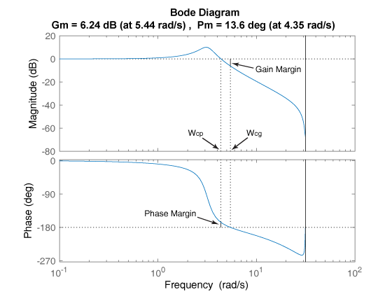
Compute the gain margin, phase margin and frequencies.
[Gm,Pm,Wcg,Wcp] = margin(sys)
Gm =
2.0519
Pm =
13.5711
Wcg =
5.4376
Wcp =
4.3544
The results indicate that a gain variation of over 2.05 (6.24 dB) at the phase crossover frequency of 5.43 rad/s would cause the system to be unstable. Similarly a phase variation of over 13.57 degrees at the gain crossover frequency of 4.35 rad/s will cause the system to lose stability.
Since R2024a
In some applications, you might want to compute stability margins within a certain frequency range, neglecting dynamics outside this range. For instance, consider the following system, with dynamics at both relatively low frequencies and relatively high frequencies.
sys = tf(5,[1 1 10]) + tf(5e3,[1 20 1e4]);
damp(sys)
         Pole              Damping       Frequency      Time Constant
                                       (rad/seconds)      (seconds)

 -5.00e-01 + 3.12e+00i     1.58e-01       3.16e+00         2.00e+00
 -5.00e-01 - 3.12e+00i     1.58e-01       3.16e+00         2.00e+00
 -1.00e+01 + 9.95e+01i     1.00e-01       1.00e+02         1.00e-01
 -1.00e+01 - 9.95e+01i     1.00e-01       1.00e+02         1.00e-01
The stability of the closed-loop system CL = feedback(sys,1) against perturbations at low frequency can be different from that at higher frequencies. To see the difference, use the Focus option. First, examine the margins below 10 rad/s.
[GmL,PmL,WcgL,WcpL] = margin(sys,Focus=[0 10])
GmL =
Inf
PmL =
80.9920
WcgL =
NaN
WcpL =
3.5137
Examine the margins about 10 rad/s.
[GmH,PmH,WcgH,WcpH] = margin(sys,Focus=[10 Inf])
GmH =
Inf
PmH =
28.6538
WcgH =
NaN
WcpH =
119.9527
For this example, load the frequency response data of an open loop system, consisting of magnitudes (m) and phase values (p) measured at the frequencies in w.
load('openLoopFRD.mat','p','m','w');
Compute the gain and phase margins.
[Gm,Pm,Wcg,Wcp] = margin(m,p,w)
Warning: The closed-loop system is unstable.
Gm =
0.6249
Pm =
48.9853
Wcg =
1.2732
Wcp =
1.5197
For this example, load invertedPendulumArray.mat, which contains a 3-by-3 array of inverted pendulum models. The mass of the pendulum varies as you move from model to model along a single column of sys, and the length of the pendulum varies as you move along a single row. The mass values used are 100g, 200g and 300g, and the pendulum lengths used are 3m, 2m and 1m respectively.
load('invertedPendulumArray.mat','sys');
size(sys)
3x3 array of transfer functions.
Each model has 1 outputs and 1 inputs.
Find gain and phase margin for all models in the array.
[Gm,Pm] = margin(sys)
Gm = 3×3

    0.9800    0.9800    0.9800
    0.9800    0.9800    0.9800
    0.9800    0.9800    0.9800
Pm = 3×3

  -11.3800  -11.4120  -11.4435
  -11.4061  -11.4298  -11.4534
  -11.4230  -11.4412  -11.4594
margin returns two arrays, Gm and Pm, in which each entry is the gain and phase margin values of the corresponding entry in sys. For instance, the gain and phase margin of the model with 100g pendulum weight and 2m length is Gm(1,2) and Pm(1,2), respectively.
Input Arguments
Output Arguments
Tips
When you use
margin(mag,phase,w),marginrelies on interpolation to approximate the margins, which generally produce less accurate results. For example, if there is no 0-dB crossing within thewrange,marginreturns a phase margin ofInf. Therefore, if you have an analytical modelsys, using[Gm,Pm,Wcg,Wcp] = margin(sys)is a more robust way to obtain the margins.If you have Robust Control Toolbox™ software, you can use
diskmargin(Robust Control Toolbox) to compute disk-based margins that define a range of "safe" gain and phase variations for which the feedback loop remains stable.
Version History
Introduced before R2006aSee Also
bode | allmargin | diskmargin (Robust Control Toolbox) | Linear System Analyzer