Multilabel Image Classification Using Deep Learning
This example shows how to use transfer learning to train a deep learning model for multilabel image classification.
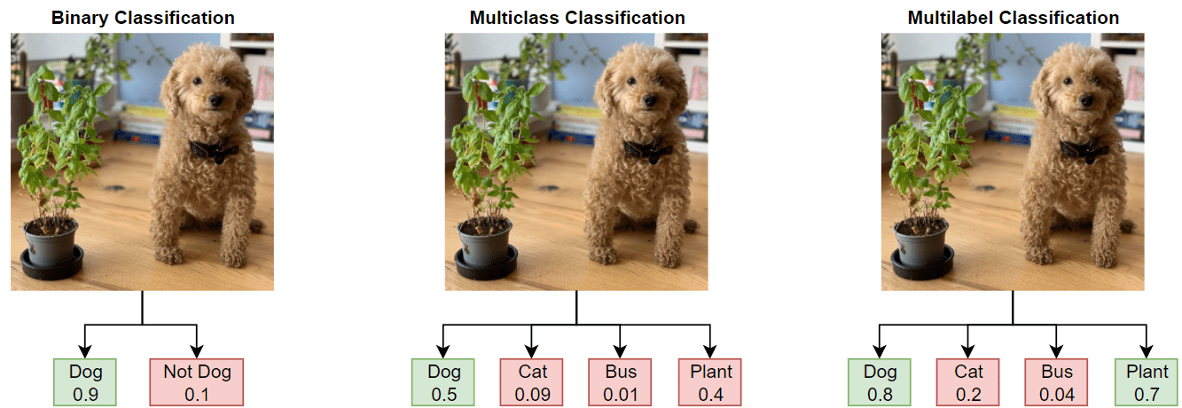
In binary or multiclass classification, a deep learning model classifies images as belonging to one of two or more classes. The data used to train the network often contains clear and focused images, with a single item in frame and without background noise or clutter. This data is often not an accurate representation of the type of data the network will receive during deployment. Additionally, binary and multiclass classification can apply only a single label to each image, leading to incorrect or misleading labeling.
In this example, you train a deep learning model for multilabel image classification by using the COCO data set, which is a realistic data set containing objects in their natural environments. The COCO images have multiple labels, so an image depicting a dog and a cat has two labels.
In multilabel classification, in contrast to binary and multiclass classification, the deep learning model predicts the probability of each class. The model has multiple independent binary classifiers, one for each class—for example, "Cat" and "Not Cat" and "Dog" and "Not Dog."
Load Pretrained Network
Load a pretrained ResNet-50 network. If the Deep Learning Toolbox Model for ResNet-50 Network support package is not installed, then the software provides a download link. ResNet-50 is trained on more than a million images and can classify images into 1000 object categories, such as keyboard, mouse, pencil, and many animals. This example uses transfer learning to retrain a ResNet-50 pretrained network for multilabel classification. For a list of all available networks, see Pretrained Deep Neural Networks.
Load the pretrained network and adapt the network for classifying 12 classes.
numClasses = 12;
net = imagePretrainedNetwork("resnet50",NumClasses=numClasses);
Extract the image input size.
inputSize = net.Layers(1).InputSize;
Prepare Data
Download and extract the COCO 2017 training and validation images and their labels from https://cocodataset.org/#download by clicking the "2017 Train images", "2017 Val images", and "2017 Train/Val annotations" links. Save the data in a folder named "COCO". The COCO 2017 data set was collected by Coco Consortium. Depending on your internet connection, the download process can take time.
Train the network on a subset of the COCO data set. For this example, train the network to recognize 12 different categories: dog, cat, bird, horse, sheep, cow, bear, giraffe, zebra, elephant, potted plant, and couch.
categoriesTrain = ["dog" "cat" "bird" "horse" "sheep" "cow" "bear" "giraffe" "zebra" "elephant" "potted plant" "couch"];
Specify the location of the training data.
dataFolder = fullfile(tempdir,"COCO");
labelLocationTrain = fullfile(dataFolder,"annotations_trainval2017","annotations","instances_train2017.json");
imageLocationTrain = fullfile(dataFolder,"train2017");
Use the supporting function prepareData, defined at the end of this example, to prepare the data for training.
Extract the labels from the file
labelLocationTrainusing thejsondecodefunction.Find the images that belong to the classes of interest.
Find the number of unique images. Many images have more than one of the class labels and, therefore, appear in the image lists for multiple categories.
Create the one-hot encoded category labels by comparing the image ID with the lists of image IDs for each category.
Create an augmented image datastore containing the images and an image augmentation scheme.
[dataTrain,encodedLabelTrain] = prepareData(labelLocationTrain,imageLocationTrain,categoriesTrain,inputSize,true);
numObservations = dataTrain.NumObservations
numObservations = 30492
The training data contains 30,492 images from 12 classes. Each image has a binary label that indicates whether it belongs to each of the 12 classes.
Prepare the validation data in the same way as the training data.
labelLocationVal = fullfile(dataFolder,"annotations_trainval2017","annotations","instances_val2017.json");
imageLocationVal = fullfile(dataFolder,"val2017");

[dataVal,encodedLabelVal] = prepareData(labelLocationVal,imageLocationVal,categoriesTrain,inputSize,false);
Inspect Data
View the number of labels for each class.
numObservationsPerClass = sum(encodedLabelTrain,1);

figure
bar(numObservationsPerClass)
ylabel("Number of Observations")
xticklabels(categoriesTrain)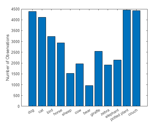
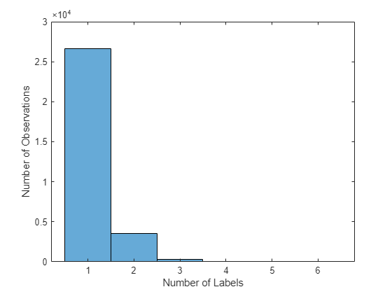
View the average number of labels per image.
numLabelsPerObservation = sum(encodedLabelTrain,2);
mean(numLabelsPerObservation)
ans = 1.1352
figure
histogram(numLabelsPerObservation)
hold on
ylabel("Number of Observations")
xlabel("Number of Labels")
hold off
Training Options
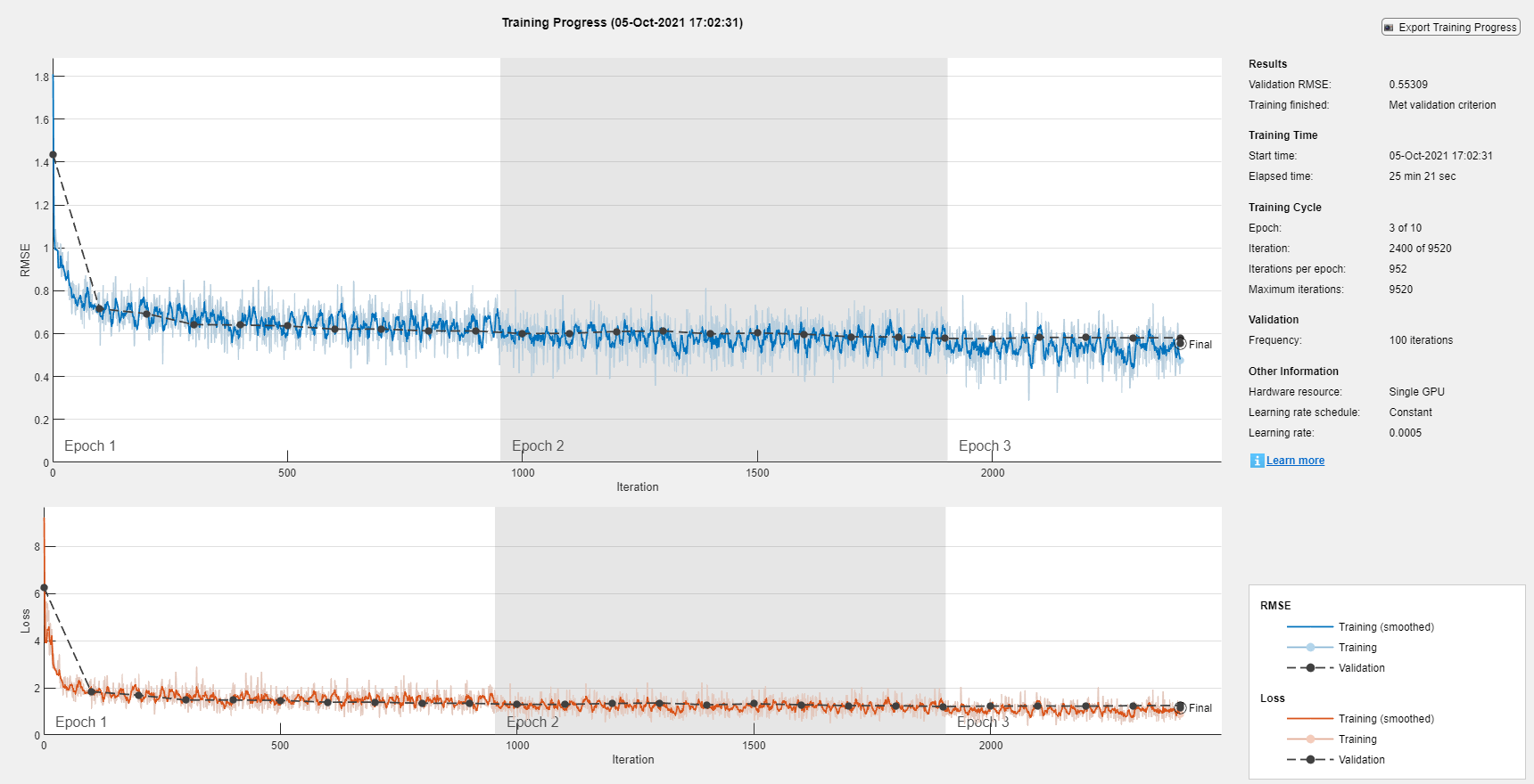
Specify the options to use for training. Train using an SGDM solver with an initial learning rate of 0.0005. Set the mini-batch size to 32 and train for a maximum of 10 epochs. Specify the validation data and set training to stop once the validation loss fails to decrease for five consecutive evaluations. Display the training progress in a plot and monitor the root mean squared error.
options = trainingOptions("sgdm", ...
    InitialLearnRate=0.0005, ...
    MiniBatchSize=32, ...
    MaxEpochs=10, ...
    Verbose= false, ...
    ValidationData=dataVal, ...
    ValidationFrequency=100, ...
    ValidationPatience=5, ...
    Metrics="rmse", ...
    Plots="training-progress");
Train Network
To save time while running this example, load a trained network and covert it to a dlnetwork object by setting doTraining to false.
To train the network yourself, set doTraining to true and train the neural network using the trainnet function. For multilabel classification, use binary-crossentropy loss. The training plot displays the RMSE and the loss. For this example, the loss is a more useful measure of network performance. By default, the trainnet function uses a GPU if one is available. Training on a GPU requires a Parallel Computing Toolbox™ license and a supported GPU device. For information on supported devices, see GPU Computing Requirements (Parallel Computing Toolbox). Otherwise, the trainnet function uses the CPU. To specify the execution environment, use the ExecutionEnvironment training option.
doTraining = false;

if doTraining
    trainedNet = trainnet(dataTrain,net,"binary-crossentropy",options);
else
    filename = matlab.internal.examples.downloadSupportFile("nnet", ...
        "data/multilabelImageClassificationNetwork.zip");

    filepath = fileparts(filename);
    dataFolder = fullfile(filepath,"multilabelImageClassificationNetwork");
    unzip(filename,dataFolder);
    load(fullfile(dataFolder,"multilabelImageClassificationNetwork.mat"));
    trainedNet = dag2dlnetwork(trainedNet);
end
Assess Model Performance
Assess the model performance on the validation data.
The model predicts the probability of each class being present in the input image. To use these probabilities to predict the classes of the image, you must define a threshold value. The model predicts that the image contains the classes with probabilities that exceed the threshold.
The threshold value controls the rate of false positives versus false negatives. Increasing the threshold reduces the number of false positives, whereas decreasing the threshold reduces the number of false negatives. Different applications will require different threshold values. For this example, set a threshold value of 0.5.
thresholdValue = 0.5;
Make predictions using the minibatchpredict function to compute the class scores for the validation data.
scores = minibatchpredict(trainedNet,dataVal);
Convert the scores to a set of predicted classes using the threshold value.
YPred = double(scores >= thresholdValue);
F1-score
Two common metrics for accessing model performance are precision (also known as the positive predictive value) and recall (also known as sensitivity).
For multilabel tasks, you can calculate the precision and recall for each class independently and then take the average (known as macro-averaging) or you can calculate the global number of true positives, false positives, and false negatives and use those values to calculate the overall precision and recall (known as micro-averaging). Throughout this example, use the micro-precision and the micro-recall values.
To combine the precision and recall into a single metric, compute the F1-score [1]. The F1-score is commonly used for evaluating model accuracy.
A value of 1 indicates that the model performs well. Use the supporting function F1Score to compute the micro-average F1-score for the validation data.
FScore = F1Score(encodedLabelVal,YPred)
FScore = 0.8158
Jaccard Index
Another useful metric for assessing performance is the Jaccard index, also known as intersection over union. This metric compares the proportion of correct labels to the total number of labels. Use the supporting function jaccardIndex to compute the Jaccard index for the validation data.
jaccardScore = jaccardIndex(encodedLabelVal,YPred)
jaccardScore = 0.7092
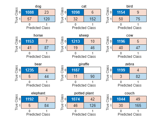
Confusion Matrix
To investigate performance at the class level, for each class, compute the confusion chart using the predicted and true binary labels.
figure
tiledlayout("flow")
for i = 1:numClasses
    nexttile
    confusionchart(encodedLabelVal(:,i),YPred(:,i));
    title(categoriesTrain(i))
end
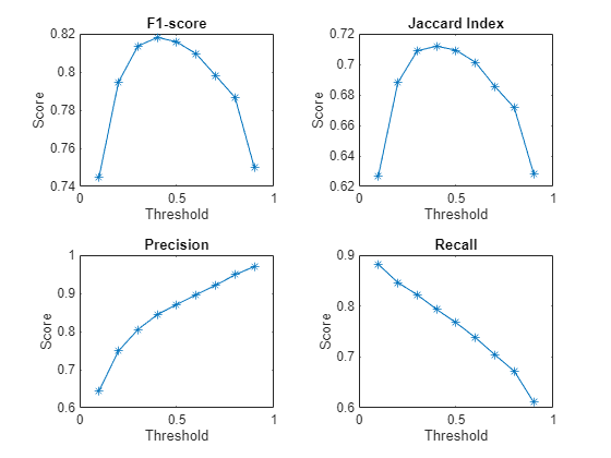
Investigate Threshold Value
Investigate how the threshold value impacts the model assessment metrics. Calculate the F1-score and the Jaccard index for different threshold values. Additionally, use the supporting function performanceMetrics to calculate the precision and recall for different threshold values.
thresholdRange = 0.1:0.1:0.9;

metricsName = ["F1-score","Jaccard Index","Precision","Recall"];
metrics = zeros(4,length(thresholdRange));

for i = 1:length(thresholdRange)

    YPred = double(scores >= thresholdRange(i));

    metrics(1,i) = F1Score(encodedLabelVal,YPred);
    metrics(2,i) = jaccardIndex(encodedLabelVal,YPred);

    [precision, recall] = performanceMetrics(encodedLabelVal,YPred);
    metrics(3,i) = precision;
    metrics(4,i) = recall;
end
Plot the results.
figure
tiledlayout("flow")
for i = 1:4
nexttile
plot(thresholdRange,metrics(i,:),"-*")
title(metricsName(i))
xlabel("Threshold")
ylabel("Score")
end
Predict Using New Data
Test the network performance on new images that are not from the COCO data set. The results indicate whether the model can generalize to images from a different underlying distribution.
imageNames = ["testMultilabelImage1.png" "testMultilabelImage2.png"];
Predict the labels for each image and view the results.
figure
tiledlayout(1,2)
images = [];
labels = [];
scores =[];

for i = 1:2
    img = imread(imageNames(i));
    img = imresize(img,inputSize(1:2));
    images{i} = img;

    scoresImg = predict(trainedNet,single(img))';
    YPred =  categoriesTrain(scoresImg >= thresholdValue);

    nexttile
    imshow(img)
    title(YPred)

    labels{i} = YPred;
    scores{i} = scoresImg;
end

Investigate Network Predictions
To further explore the network predictions, you can use visualization methods to highlight which area of an image the network is using when making the class predictions. Grad-CAM is a visualization method that uses the gradient of the class scores with respect to the convolutional features determined by the network to understand which parts of the image are most important for each class label. The places where this gradient is large are exactly the places where the final score depends most on the data.
Investigate the first image. The network correctly identifies the cat and couch in this image. However, the network fails to identify the dog.
imageIdx = 1;
testImage = images{imageIdx};
Generate a table containing the scores for each class.
tbl = table(categoriesTrain',scores{imageIdx},VariableNames=["Class", "Score"]);
disp(tbl)
Class Score
______________ __________
"dog" 0.18477
"cat" 0.88647
"bird" 6.2184e-05
"horse" 0.0020663
"sheep" 0.00015361
"cow" 0.00077924
"bear" 0.0016855
"giraffe" 2.5157e-06
"zebra" 8.097e-05
"elephant" 9.5033e-05
"potted plant" 0.0051869
"couch" 0.80556
The network is confident that this image contains a cat and a couch but less confident that the image contains a dog. Use Grad-CAM to see which parts of the image the network is using for each of the true classes.
targetClasses = ["dog","cat","couch"];
targetClassesIdx = find(ismember(categoriesTrain,targetClasses));
Generate the Grad-CAM map for each class label.
reductionLayer = "sigmoid";
map = gradCAM(trainedNet,testImage,targetClassesIdx,ReductionLayer=reductionLayer);
Plot the Grad-CAM results as an overlay on the image.
figure
tiledlayout("flow")

nexttile
imshow(testImage)
for i = 1:length(targetClasses)
    nexttile
    imshow(testImage)
    hold on
    title(targetClasses(i))
    imagesc(map(:,:,i),AlphaData=0.5)
    hold off
end
colormap jet
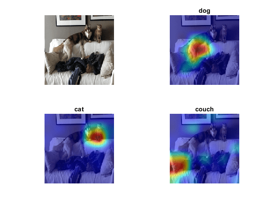
The Grad-CAM maps show that the network is correctly identifying the objects in the image.
Supporting Functions
Prepare Data
The supporting function prepareData prepares the COCO data for multilabel classification training and prediction.
Extract the labels from the file
labelLocationusing thejsondecodefunction.Find the images that belong to the classes of interest.
Find the number of unique images. Many images have more than one of the given labels and appear in the image lists for multiple categories.
Create the one-hot encoded category labels by comparing the image ID with the lists of image IDs for each category.
Combine the data and one-hot encoded labels into a table.
Create an augmented image datastore containing the image. Turn grayscale images into RGB images.
The prepareData function uses the COCOImageID function (attached as a supporting file). To access this function, open this example as a live script.
function [data, encodedLabel] = prepareData(labelLocation,imageLocation,categoriesTrain,inputSize,doAugmentation)

miniBatchSize = 32;

% Extract labels.
strData = fileread(labelLocation);
dataStruct = jsondecode(strData);

numClasses = length(categoriesTrain);

% Find images that belong to the subset categoriesTrain using
% the COCOImageID function, attached as a supporting file.
images = cell(numClasses,1);
for i=1:numClasses
    images{i} = COCOImageID(categoriesTrain(i),dataStruct);
end

% Find the unique images.
imageList = [images{:}];
imageList = unique(imageList);
numUniqueImages = numel(imageList);

% Encode the labels.
encodedLabel = zeros(numUniqueImages,numClasses);
imgFiles = strings(numUniqueImages,1);
for i = 1:numUniqueImages
    imgID = imageList(i);
    imgFiles(i) = fullfile(imageLocation + "\" + pad(string(imgID),12,"left","0") + ".jpg");

    for j = 1:numClasses
        if ismember(imgID,images{j})
            encodedLabel(i,j) = 1;
        end
    end
end

% Define the image augmentation scheme.
imageAugmenter = imageDataAugmenter( ...
    RandRotation=[-45,45], ...
    RandXReflection=true);

% Store the data in a table.
dataTable = table(Size=[numUniqueImages 2], ...
    VariableTypes=["string" "double"], ...
    VariableNames=["File_Location" "Labels"]);

dataTable.File_Location = imgFiles;
dataTable.Labels = encodedLabel;

% Create a datastore. Transform grayscale images into RGB.
if doAugmentation
    data = augmentedImageDatastore(inputSize(1:2),dataTable, ...
        ColorPreprocessing="gray2rgb", ...
        DataAugmentation=imageAugmenter);
else
    data = augmentedImageDatastore(inputSize(1:2),dataTable, ...
        ColorPreprocessing="gray2rgb");
end
data.MiniBatchSize = miniBatchSize;
end
F1-score
The supporting function F1Score computes the micro-averaging F1-score [1].
function score = F1Score(T,Y)
% TP: True Positive
% FP: False Positive
% TN: True Negative
% FN: False Negative

TP = sum(T .* Y,"all");
FP = sum(Y,"all")-TP;

TN = sum(~T .* ~Y,"all");
FN = sum(~Y,"all")-TN;

score = TP/(TP + 0.5*(FP+FN));
end
Jaccard Index
The supporting function jaccardIndex computes the Jaccard index, also called intersection over union, as given by
,
where T and Y correspond to the targets and predictions. The Jaccard index describes the proportion of correct labels compared to the total number of labels.
function score = jaccardIndex(T,Y)

intersection = sum((T.*Y));

union = T+Y;
union(union < 0) = 0;
union(union > 1) = 1;
union = sum(union);

% Ensure the accuracy is 1 for instances where a sample does not belong to any class
% and the prediction is correct. For example, T = [0 0 0 0] and Y = [0 0 0 0].
noClassIdx = union == 0;
intersection(noClassIdx) = 1;
union(noClassIdx) = 1;

score = mean(intersection./union);
end
Precision and Recall
Two common metrics for model assessment are precision (also known as the positive predictive value) and recall (also known as sensitivity).
The supporting function performanceMetrics calculates the micro-average precision and recall values.
function [precision, recall] = performanceMetrics(T,Y)
% TP: True Positive
% FP: False Positive
% TN: True Negative
% FN: False Negative

TP = sum(T .* Y,"all");
FP = sum(Y,"all")-TP;

TN = sum(~T .* ~Y,"all");
FN = sum(~Y,"all")-TN;

precision = TP/(TP+FP);
recall = TP/(TP+FN);
end
References
[1] Sokolova, Marina, and Guy Lapalme. "A Systematic Analysis of Performance Measures for Classification Tasks." Information Processing & Management 45, no. 4 (2009): 427–437.
See Also
gradCAM | imagePretrainedNetwork | trainnet | trainingOptions | dlnetwork