dsp.FIRRateConverter
Perform polyphase FIR sample rate conversion
Description
The dsp.FIRRateConverter
System object™ performs an efficient polyphase sample rate conversion using a rational factor
L/M along the first dimension.
The FIR rate converter cascades an interpolator with a decimator. Conceptually, the rate
converter (as shown in the schematic) consists of an upsampler, followed by a combined
anti-imaging and anti-aliasing FIR filter, followed by a downsampler. The coefficients of the
anti-imaging and anti-aliasing FIR filter can be specified through the
Numerator property, or can be automatically designed by the object
using the designMultirateFIR function. For an example, see
Resample Signal Using FIR Rate Converter.
The upsampler increases the sample rate of the signal by a factor L and the downsampler reduces the sample rate of the signal by a factor M. Use upsampling and downsampling factors that are relatively prime or coprime. The resulting discrete-time signal has a sample rate that is L/M times the original sample rate.

Note that the actual object algorithm implements a polyphase structure, an efficient equivalent of the combined system depicted in the diagram. For more details, see Algorithms.
To perform sampling rate conversion:
Create the
dsp.FIRRateConverterobject and set its properties.Call the object with arguments, as if it were a function.
To learn more about how System objects work, see What Are System Objects?
Creation
Syntax
Description
firrc = dsp.FIRRateConverterdesignMultirateFIR(3,2) function.
firrc = dsp.FIRRateConverter(L,M)InterpolationFactor property set to L and the
DecimationFactor property set to M. The object
designs its filter coefficients based on the rate conversion factors that you specify
while creating the object, using the designMultirateFIR(L,M)
function. The designed filter corresponds to a lowpass filter with normalized cutoff
frequency no greater than min(π/L,π/M) in radial frequency
units.
firrc = dsp.FIRRateConverter(L,M,"Auto")NumeratorSource property is set to
"Auto". In this mode, every time there is an
update in the rate conversion factors, the object redesigns the filter
using the design method specified in
DesignMethod.
firrc = dsp.FIRRateConverter(L,M,num)Numerator property set
to num.
firrc = dsp.FIRRateConverter(L,M,method)DesignMethod property set to
method. When you pass the design method as an
input, the NumeratorSource property is
automatically set to "Auto".
firrc = dsp.FIRRateConverter(___,InputSampleRate=Value)"normalized". (since R2026a)
To specify an input sample rate of 22050 Hz, set
InputSampleRate to 22050. To specify the input sample rate in
normalized units, set InputSampleRate to
"normalized". (since R2026a)
firrc = dsp.FIRRateConverter(___,PropertyName=Value)
Example: firrc =
dsp.FIRRateConverter(FullPrecisionOverride="false")
enables the fixed-point data types to be controlled through the
individual fixed-point property settings.
firrc = dsp.FIRRateConverter(L,M,"legacy")firpm(70,[0 0.28 0.32 1],[1 1 0
0]). The designed filter has a cutoff frequency of π/3
radians/sample.
Properties
Usage
Syntax
Input Arguments
Output Arguments
Object Functions
To use an object function, specify the
System object as the first input argument. For
example, to release system resources of a System object named obj, use
this syntax:
release(obj)
Examples
Resample a 100 Hz sine wave signal by a factor of 3/2.
Create a dsp.SineWave object which generates a sinusoidal signal with 54 samples per frame, contains a tone at 100 Hz, and has a sample rate of 1250 Hz.
sine = dsp.SineWave(1,100,SampleRate=1250,SamplesPerFrame=54);

% Grab a frame
x = sine();

% Calculate input time vector
tx = (0:length(x)-1)/sine.SampleRate;
Design Default Filter
Create a dsp.FIRRateConverter object. The object uses a combined anti-imaging and anti-aliasing FIR filter. By default, this filter is designed using the designMultirateFIR function. The function designs the filter based on the rate conversion factors that you specify, and stores the coefficients in the Numerator property. For an interpolation factor of 3 and a decimation factor of 2, the object designs the coefficients using designMultirateFIR(3,2).
firrc = dsp.FIRRateConverter(3,2);
Resample by a Factor of 3/2
Resample the signal by a factor of 3/2.
y = firrc(x);
Plot the original and resampled signals. In order to plot the two signals on the same plot, you must account for the output delay of the FIR rate converter and the scaling introduced by the filter. Use the outputDelay function to compute the delay value introduced by the rate converter. Shift the output by this delay value.
Visualize the input and the resampled signals. The input and output values coincide every 3 output samples, and every other input sample, owing to the conversion rate of 3/2.
FsIn = sine.SampleRate;
[delay,FsOut] = outputDelay(firrc,InputSampleRate=FsIn);
% Calculate output times for vector y in input units
ty = (0:length(y)-1)/FsOut-delay;

stem(tx,x,"filled",MarkerSize=4)
hold on
stem(ty,y)
hold off
xlim([0.0 0.0145])
ylim([-1.5 1.5])
legend("Original input","Resampled")

Resample by a Factor of 5/3 in Automatic Filter Design Mode
Now change the interpolation factor to 5 and the decimation factor to 3. In order for the filter design to be updated automatically based on the new rate conversion factors, set the NumeratorSource property to "Auto". Alternately, you can pass the keyword "auto" as an input while creating the object. The object then operates in the automatic filter design mode. Every time there is a change in the rate conversion factors, the object updates the filter design accordingly.
release(firrc)
firrc.NumeratorSource = "Auto";
firrc.InterpolationFactor = 5;
firrc.DecimationFactor = 3
firrc =
dsp.FIRRateConverter with properties:
Main
InterpolationFactor: 5
DecimationFactor: 3
NumeratorSource: 'Auto'
DesignMethod: 'Kaiser'
Show all properties
To access the filter coefficients in the automatic filter design mode, type firrc.Numerator in the MATLAB command prompt.
Resample the signal with the updated rate conversion values.
yAuto = firrc(x);
Plot the original and resampled signals. Recalculate the output delay and the output sample rate since the rate conversion factors have changed. Note that the input and output coincide every 3 input samples, and every 5 output samples, owing to the 5/3 conversion factor.
[delay,FsOut] = outputDelay(firrc,InputSampleRate=FsIn);
% Calculate output times for vector yAuto in input units
tyAuto = (0:length(yAuto)-1)/FsOut-delay;

stem(tx,x,"filled",MarkerSize=4)
hold on
stem(tyAuto,yAuto,"r")
hold off
xlim([0.0 0.015])
ylim([-1.5 1.5])
legend("Original input","Resampled")

Specify Signal Interpolation Model
In the automatic design mode, you can also specify the underlying D/A signal interpolation model through the DesignMethod property.
Set DesignMethod to "linear" and change the interpolation factor to 11.
release(firrc)
firrc.InterpolationFactor = 11;
firrc.DesignMethod = "linear";
Resample the signal using the linear interpolation model.
yLinear = firrc(x);
Plot the original and resampled signals. The output samples lie on a piecewise-linear curve. Note that the input and output coincide every three input samples and every 11 output samples as expected from the ratio 11/3.
[delay,FsOut] = outputDelay(firrc,InputSampleRate=FsIn);
% Calculate output times for vector yLinear in input units
tyLinear = (0:length(yLinear)-1)/FsOut-delay;

stem(tx,x,"filled",MarkerSize=4)
hold on
stem(tyLinear,yLinear)
plot(tyLinear,yLinear,Color=[1 0 0 0.3])
hold off
xlim([0.0 0.009])
ylim([-1.5 1.5])
legend("Original input","Resampled")

Resample an audio signal from 48 kHz to 44 kHz and play the resampled signal using the audioDeviceWriter object.
Note: The audioDeviceWriter System object™ is not supported in MATLAB Online.
Create a dsp.AudioFileReader object. The object reads an audio file that has a sample rate of 48 kHz.
L = 11;
M = 12;
afr = dsp.AudioFileReader('audio48kHz.wav', ...
    'OutputDataType','single', ...
    'SamplesPerFrame',4*M);
Create a dsp.FIRRateConverter object with an interpolation factor of L = 11 and a decimation factor of M = 12 (the co-prime representation of the ratio ), a reasonable approximation of the standard 44.1 kHz rate. The object designs the filter using designMultirateFIR(11,12) and stores the coefficients in the Numerator property of the object.
firrc = dsp.FIRRateConverter(L,M)
firrc =
  dsp.FIRRateConverter with properties:

   Main
    InterpolationFactor: 11
       DecimationFactor: 12
        NumeratorSource: 'Property'
              Numerator: [0 2.3076e-05 5.4790e-05 9.3620e-05 1.3665e-04 1.7959e-04 2.1699e-04 2.4263e-04 2.5004e-04 2.3320e-04 1.8731e-04 1.0959e-04 0 -1.3820e-04 -2.9809e-04 -4.6908e-04 -6.3723e-04 -7.8603e-04 -8.9751e-04 -9.5372e-04 … ] (1×264 double)

  Show all properties
Create an audioDeviceWriter object. Specify the sample rate to be 44100 Hz.
adw = audioDeviceWriter(44100);
Read the audio file, convert the sample rate of the audio signal, and play the resampled audio.
while ~isDone(afr)
    audio1 = afr();
    audio2 = firrc(audio1);
    adw(audio2);
end
release(afr)
release(adw)
Since R2026a
Specify the input sample rate explicitly while constructing the dsp.FIRRateConverter object using the InputSampleRate argument.
firRC = dsp.FIRRateConverter(InputSampleRate=22050)
firRC =
  dsp.FIRRateConverter with properties:

   Main
    InterpolationFactor: 3
       DecimationFactor: 2
        NumeratorSource: 'Property'
              Numerator: [0 -1.2906e-04 -2.2804e-04 0 5.5461e-04 8.0261e-04 0 -0.0015 -0.0020 0 0.0034 0.0043 0 -0.0067 -0.0083 0 0.0121 0.0145 0 -0.0205 -0.0241 0 0.0332 0.0388 0 -0.0530 -0.0620 0 0.0861 0.1027 0 -0.1540 -0.1976 0 … ] (1×72 double)

  Show all properties
You can view this information using the Input sample rate field of the info function.
info(firRC)
ans = 13×71 char array
    'Discrete-Time FIR Multirate Filter (real)                              '
    '-----------------------------------------                              '
    'Filter Structure      : Direct-Form FIR Polyphase Sample-Rate Converter'
    'Interpolation Factor  : 3                                              '
    'Decimation Factor     : 2                                              '
    'Filter Length         : 72                                             '
    'Polyphase Length      : 24                                             '
    'Stable                : Yes                                            '
    'Linear Phase          : Yes (Type 1)                                   '
    '                                                                       '
    'Arithmetic            : double                                         '
    'Input sample rate     : 22050                                          '
    '                                                                       '
Visualize the frequency response of the filter using filterAnalyzer. Note the frequency range from 0 to 11025 Hz.
filterAnalyzer(firRC,FilterNames="InputSampleRate22050Hz")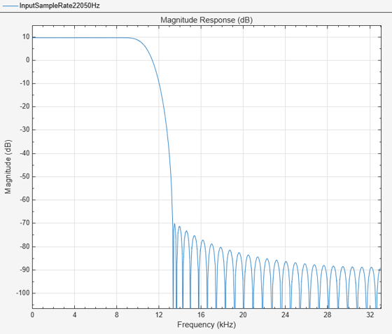
To specify the input sample rate after constructing the object, use the setInputSampleRate function.
setInputSampleRate(firRC,44100)
To confirm, view the sample rate information using the info function.
info(firRC)
ans = 13×71 char array
    'Discrete-Time FIR Multirate Filter (real)                              '
    '-----------------------------------------                              '
    'Filter Structure      : Direct-Form FIR Polyphase Sample-Rate Converter'
    'Interpolation Factor  : 3                                              '
    'Decimation Factor     : 2                                              '
    'Filter Length         : 72                                             '
    'Polyphase Length      : 24                                             '
    'Stable                : Yes                                            '
    'Linear Phase          : Yes (Type 1)                                   '
    '                                                                       '
    'Arithmetic            : double                                         '
    'Input sample rate     : 44100                                          '
    '                                                                       '
Visualize the frequency response of the filter using filterAnalyzer. Note the change in frequency interval from 0 to 22050 Hz.
filterAnalyzer(firRC,FilterNames="InputSampleRate44100Hz")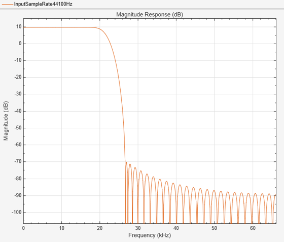
More About
Algorithms
The FIR rate converter is implemented efficiently using a polyphase structure.
To derive the polyphase structure, start with the transfer function of the FIR filter: This FIR filter is a combined anti-imaging and anti-aliasing filter.
N+1 is the length of the FIR filter.
You can rearrange this equation as follows:
L is the number of polyphase components, and its value equals the interpolation factor that you specify.
You can write this equation as:
E0(zL), E1(zL), ..., EL-1(zL) are polyphase components of the FIR filter H(z).
Conceptually, the FIR rate converter contains an upsampler, followed by a combined anti-imaging, anti-aliasing FIR filter H(z), which is followed by a downsampler.

Replace H(z) with its polyphase representation.

Here is the multirate noble identity for interpolation.

Applying the noble identity for interpolation moves the upsampling operation to after the filtering operation. This move enables you to filter the signal at a lower rate.

You can replace the upsampling operator, delay block, and the adder with a commutator switch. To account for the downsampler that follows, the switch moves in steps of size M. The switch receives the first sample from branch 0 and moves in the counter clockwise direction, each time skipping M−1 branches.
As an example, consider a rate converter with L set to 5 and M set to 3. The polyphase components are E0(z), E1(z), E2(z), E3(z), and E4(z). The switch starts on the first branch 0, skips branches 1 and 2, receives the next sample from branch 3, then skips branches 4 and 0, receives the next sample from branch 2, and so on. The sequence of branches from which the switch receives the data sample is [0, 3, 1, 4, 2, 0, 3, 1, ….].
The rate converter implements the L/M conversion by first applying the interpolation factor L to the incoming data, and using the commutator switch at the end to receive only 1 in M samples, effectively accounting for the downsampling factor M. Hence, the sample rate at the output of the FIR rate converter is Lfs/M.

Extended Capabilities
Version History
Introduced in R2012aSee Also
Functions
freqz|freqzmr|filterAnalyzer|info|cost|coeffs|polyphase|outputDelay|designRateConverter|setInputSampleRate