Main Content

freqsamp

Real or complex frequency-sampled FIR filter from specification object

Syntax

hd = design(d,'freqsamp','SystemObject',true)
hd = design(...,'filterstructure',structure,'SystemObject',true)
hd = design(...,'window',window,'SystemObject',true)

Description

hd = design(d,'freqsamp','SystemObject',true) designs a frequency-sampled filter specified by the filter specifications object d.

hd = design(...,'filterstructure',structure,'SystemObject',true) returns a filter with the filter structure you specify by the structure input argument. structure is dffir by default and can be any one of the following filter structures.

Structure

Description of Resulting Filter Structure

dffir

Direct-form FIR filter

dffirt

Transposed direct-form FIR filter

dfsymfir

Symmetrical direct-form FIR filter

dfasymfir

Asymmetrical direct-form FIR filter

hd = design(...,'window',window,'SystemObject',true) designs filters using the window specified by window. Provide the input argument window as

  • A character vector for the window type. For example, use 'bartlett', or 'hamming'. See window for the full list of windows available.

  • A function handle that references the window function. When the window function requires more than one input, use a cell array to hold the required arguments. The first example shows a cell array input argument.

  • The window vector itself.

Examples

collapse all

These examples design FIR filters that have arbitrary magnitude responses. In the first filter, the response has three distinct sections and the resulting filter is real.

The second example creates a complex filter.

b1 = 0:0.01:0.18;
b2 = [.2 .38 .4 .55 .562 .585 .6 .78];
b3 = 0.79:0.01:1;
a1 = .5+sin(2*pi*7.5*b1)/4;    % Sinusoidal response section.
a2 = [.5 2.3 1 1 -.2 -.2 1 1]; % Piecewise linear response section.
a3 = .2+18*(1-b3).^2;          % Quadratic response section.
f = [b1 b2 b3];
a = [a1 a2 a3];
n = 300;
d = fdesign.arbmag('n,f,a',n,f,a); % First specifications object.
hd = design(d,'freqsamp','window',{@kaiser,.5},...
    'SystemObject',true); % Filter.
filterAnalyzer(hd)

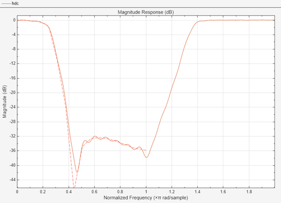
Now design the arbitrary-magnitude complex FIR filter. Recall that vector f contains frequency locations and vector a contains the desired filter response values at the locations specified in f.

f = [-1 -.93443 -.86885 -.80328 -.7377 -.67213 -.60656 -.54098 ...
-.47541,-.40984 -.34426 -.27869 -.21311 -.14754 -.081967 ...
-.016393 .04918 .11475,.18033 .2459 .31148 .37705 .44262 ...
 .5082 .57377 .63934 .70492 .77049,.83607 .90164 1];
a = [.0095848 .021972 .047249 .099869 .23119 .57569 .94032 ...
.98084 .99707,.99565 .9958 .99899 .99402 .99978 .99995 .99733 ...
.99731 .96979 .94936,.8196 .28502 .065469 .0044517 .018164 ...
.023305 .02397 .023141 .021341,.019364 .017379 .016061];
n = 48;
d = fdesign.arbmag('n,f,a',n,f,a); % Second spec. object.
hdc = design(d,'freqsamp','window','rectwin',SystemObject=true); % Filter
filterAnalyzer(hdc)

The response for hdc is from -1 to 1 in normalized frequency. design(d,...) returns a complex filter for hdc because the frequency vector includes negative frequency values.

Version History

Introduced in R2011a

Go to top of page