Compute State Distribution of Markov Chain at Each Time Step
This example shows how to compute and visualize state redistributions, which show the evolution of the deterministic state distributions over time from an initial distribution.
Consider this theoretical, right-stochastic transition matrix of a stochastic process.
Create the Markov chain that is characterized by the transition matrix P.
P = [ 0   0  1/2 1/4 1/4  0   0 ;
      0   0  1/3  0  2/3  0   0 ;
      0   0   0   0   0  1/3 2/3;
      0   0   0   0   0  1/2 1/2;
      0   0   0   0   0  3/4 1/4;
     1/2 1/2  0   0   0   0   0 ;
     1/4 3/4  0   0   0   0   0 ];
mc = dtmc(P);
Plot a directed graph of the Markov chain and identify classes using node colors and markers.
figure
graphplot(mc,ColorNodes=true)
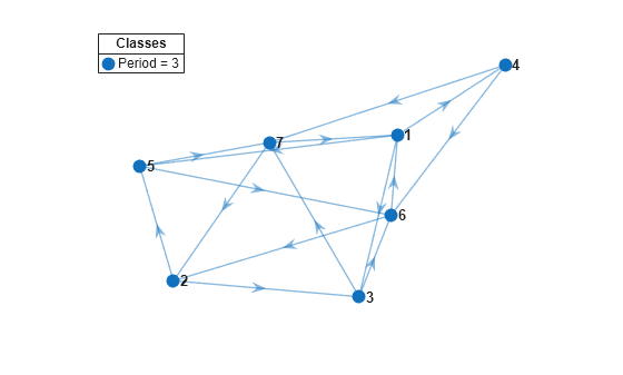
mc represents a single recurrent class with a period of 3.
Suppose that the initial state distribution is uniform. Compute the evolution of the distribution for 20 time steps.
numSteps = 20;
X = redistribute(mc,numSteps);
X is a 21-by-7 matrix. Row t contains the evolved state distribution at time step t.
Visualize the redistributions in a heatmap.
figure
distplot(mc,X)
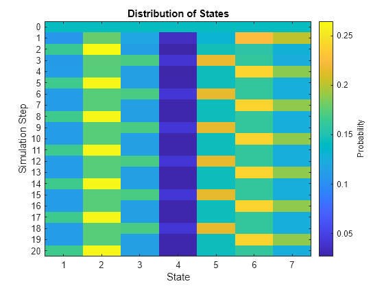
The periodicity of the chain is apparent.
Remove the periodicity from the Markov chain by transforming it to a lazy chain. Plot a heatmap of the transition matrix of the lazy chain.
lc = lazy(mc);
figure
imagesc(lc.P)
axis square
colorbar
title("Theoretical Lazy Chain Transition Matrix")
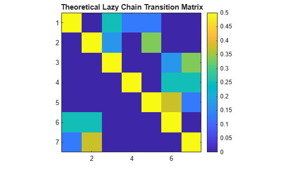
lc is a dtmc object. lazy creates the lazy chain by adding weight to the probability of persistence, that is, lazy enforces self-loops.
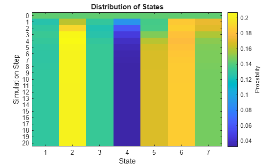
Compute the evolution of the distribution in the lazy chain for 20 time steps. Plot the redistributions in a heatmap.
X1 = redistribute(lc,numSteps);

figure
distplot(lc,X1)
View the evolution of the state distribution as an animated histogram. Specify a frame rate of 1 second.
figure
distplot(lc,X1,Type="histogram",FrameRate=1)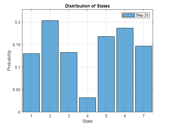
Compute the stationary distribution of the lazy chain. Compare it to the final redistribution in the animated histogram.
xFix = asymptotics(lc)
xFix = 1×7

    0.1300    0.2034    0.1328    0.0325    0.1681    0.1866    0.1468
The stationary distribution and the final redistribution are nearly identical.