Simulate Random Walks Through Markov Chain
This example shows how to generate and visualize random walks through a Markov chain.
Consider this theoretical, right-stochastic transition matrix of a stochastic process.
Create the Markov chain that is characterized by the transition matrix P.
P = [ 0   0  1/2 1/4 1/4  0   0 ;
      0   0  1/3  0  2/3  0   0 ;
      0   0   0   0   0  1/3 2/3;
      0   0   0   0   0  1/2 1/2;
      0   0   0   0   0  3/4 1/4;
     1/2 1/2  0   0   0   0   0 ;
     1/4 3/4  0   0   0   0   0 ];
mc = dtmc(P);
Plot a directed graph of the Markov chain and identify classes using node colors and markers.
figure
graphplot(mc,ColorNodes=true);
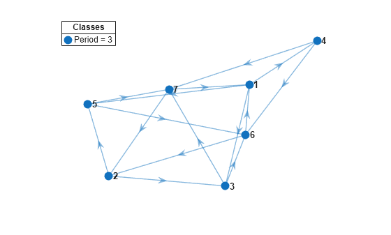
mc represents a single recurrent class with a period of 3.
Simulate one random walk of 20 steps through the chain. Start in a random initial state.
rng(1,"twister")  % For reproducibility
numSteps = 20;
X = simulate(mc,numSteps);
X is a 21-by-1 vector containing the indices of states visited during the random walk. The first row contains the realized initial state.
Plot a heatmap of the random walk.
figure
simplot(mc,X)
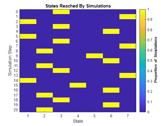
The return time to any state is a multiple of three.
Show the random walk through the Markov chain as an animation through the digraph. Specify a frame rate of 1 second.
figure
simplot(mc,X,FrameRate=1,Type="graph")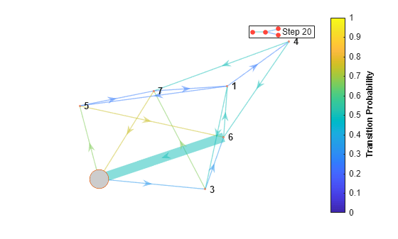
Simulate 100 random walks: 50 starting from state 1, 49 starting from state 2, and 1 starting from state 6. Plot a heatmap of the simulation.
x0 = [50 49 0 0 0 1 0];
X1 = simulate(mc,numSteps,X=x0)
X1 = 21×100

     1     1     1     1     1     1     1     1     1     1     1     1     1     1     1     1     1     1     1     1     1     1     1     1     1     1     1     1     1     1     1     1     1     1     1     1     1     1     1     1     1     1     1     1     1     1     1     1     1     1
     5     4     3     4     4     3     3     3     3     4     3     5     5     5     5     4     5     3     4     5     3     3     5     5     3     4     4     4     3     5     4     5     4     4     3     5     3     5     5     3     3     3     3     3     5     3     3     5     3     5
     6     6     7     7     7     6     6     7     7     7     6     6     7     6     6     6     7     7     7     6     6     7     6     6     6     7     6     7     7     6     6     6     6     7     7     6     6     6     6     7     7     6     7     7     6     6     7     6     7     7
     2     2     2     2     2     1     1     2     1     2     2     1     2     1     2     1     2     2     1     2     1     1     1     2     1     2     1     1     2     1     2     2     2     2     2     2     2     1     2     2     1     2     2     2     2     2     2     2     1     2
     5     3     3     3     5     5     3     3     3     5     5     5     5     3     3     4     3     5     3     5     3     5     5     5     4     5     3     4     5     3     5     5     3     5     5     5     3     3     5     5     3     5     5     5     5     5     3     3     3     5
     7     7     7     7     6     6     6     6     7     6     7     6     6     7     7     6     7     6     6     7     6     7     6     6     6     6     6     7     6     7     6     6     7     7     6     6     7     6     6     7     7     6     7     6     6     6     7     6     7     6
     1     2     2     2     1     2     1     1     1     2     2     1     2     2     2     1     2     2     2     1     1     2     2     1     2     1     2     2     2     2     2     1     2     2     2     2     2     2     2     2     2     2     2     2     2     2     2     1     2     1
     3     3     5     5     5     5     4     3     4     5     5     3     5     5     3     4     5     5     5     3     5     5     3     3     3     3     3     5     5     5     5     3     3     5     5     3     5     5     5     5     3     3     5     3     3     5     3     3     3     3
     6     6     7     6     6     6     7     7     7     7     7     7     6     6     7     7     7     6     6     6     6     6     7     7     7     7     7     6     6     6     6     7     7     6     6     7     6     7     6     6     7     7     6     7     7     6     6     7     7     6
     2     1     2     2     2     1     1     2     2     2     2     2     1     2     2     2     1     1     2     1     2     1     2     2     1     2     1     1     2     2     2     2     1     2     2     2     2     2     2     1     2     2     2     2     1     1     1     2     2     2
     3     3     5     3     3     4     3     3     3     5     5     3     3     5     5     3     5     3     3     3     5     3     5     5     4     5     3     3     3     5     3     5     5     3     3     5     5     5     5     3     5     5     3     3     4     3     3     5     5     5
     7     7     6     7     6     7     7     7     6     7     6     7     6     7     7     7     6     6     7     7     6     7     6     7     6     6     7     7     7     7     7     6     6     7     7     6     6     6     6     7     6     6     6     7     6     7     7     7     6     6
     2     1     1     2     2     2     2     2     2     1     2     2     2     2     2     1     1     1     2     2     1     2     1     2     1     2     2     2     2     2     2     2     1     2     2     2     2     2     1     2     1     2     1     2     2     1     1     2     2     2
     5     3     5     5     5     3     3     5     5     3     3     5     5     5     3     4     3     4     3     5     3     5     4     3     3     5     5     5     3     5     5     3     5     3     5     3     5     5     4     5     3     3     3     5     5     3     3     5     5     5
     6     7     6     6     6     7     6     6     7     6     7     6     7     6     6     7     7     6     7     7     7     6     7     7     7     7     6     6     6     6     7     7     6     6     7     7     6     6     6     7     7     7     7     7     7     7     6     6     6     6
      ⋮
figure
simplot(mc,X1)
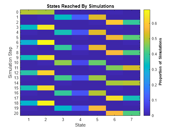
X1 is a 21-by-100 matrix of random walks. The first 50 columns correspond to the walks starting from state 1, the next 49 columns correspond to the walks starting from state 2, and the last column corresponds to the walk starting from state 6.
The three periodic subclasses are evident.
View the realized transition matrix of the 100 random walks as a heatmap.
figure
simplot(mc,X1,Type="transitions")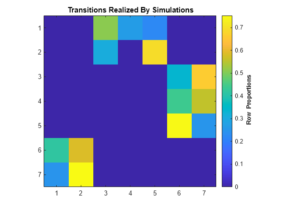
Visually compare the realized and theoretical transition matrices.
figure
imagesc(mc.P)
axis square
colorbar
title("Theoretical Transition Matrix")
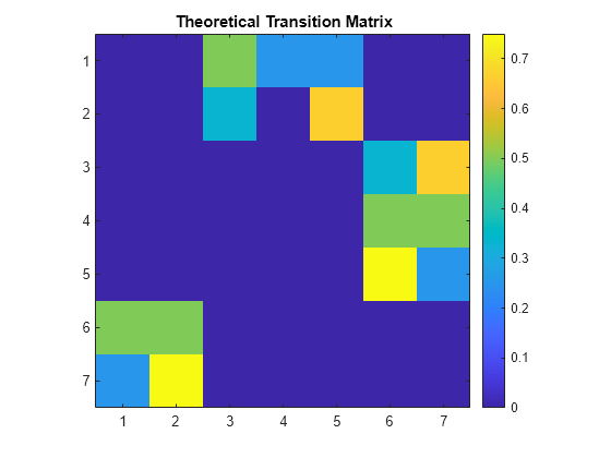
The transition matrices are similar.