Fit VAR Model of CPI and Unemployment Rate
This example shows how to estimate the parameters of a VAR(4) model. The response series are quarterly measures of the consumer price index (CPI) and the unemployment rate.
Load the Data_USEconModel data set.
load Data_USEconModelPlot the two series on separate plots.
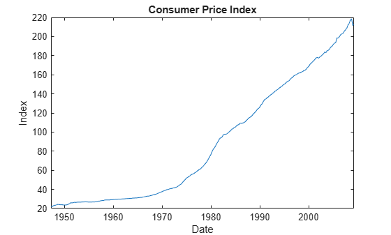
figure;
plot(DataTimeTable.Time,DataTimeTable.CPIAUCSL);
title('Consumer Price Index')
ylabel('Index')
xlabel('Date')
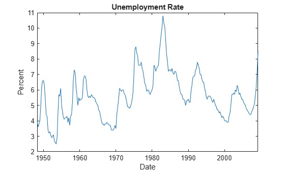
figure;
plot(DataTimeTable.Time,DataTimeTable.UNRATE);
title('Unemployment Rate')
ylabel('Percent')
xlabel('Date')
The CPI appears to grow exponentially.
Stabilize the CPI by converting it to a series of growth rates. Synchronize the two series by removing the first observation from the unemployment rate series.
rcpi = price2ret(DataTimeTable.CPIAUCSL);
unrate = DataTimeTable.UNRATE(2:end);
Create a default VAR(4) model using the shorthand syntax.
Mdl = varm(2,4)
Mdl =
  varm with properties:

     Description: "2-Dimensional VAR(4) Model"
     SeriesNames: "Y1"  "Y2"
       NumSeries: 2
               P: 4
        Constant: [2×1 vector of NaNs]
              AR: {2×2 matrices of NaNs} at lags [1 2 3 ... and 1 more]
           Trend: [2×1 vector of zeros]
            Beta: [2×0 matrix]
      Covariance: [2×2 matrix of NaNs]
Mdl is a varm model object. It serves as a template for model estimation. MATLAB� considers any NaN values as unknown parameter values to be estimated. For example, the Constant property is a 2-by-1 vector of NaN values. Therefore, model constants are model parameters to be estimated.
Fit the model to the data.
EstMdl = estimate(Mdl,[rcpi unrate])
EstMdl =
  varm with properties:

     Description: "AR-Stationary 2-Dimensional VAR(4) Model"
     SeriesNames: "Y1"  "Y2"
       NumSeries: 2
               P: 4
        Constant: [0.00171639 0.316255]'
              AR: {2×2 matrices} at lags [1 2 3 ... and 1 more]
           Trend: [2×1 vector of zeros]
            Beta: [2×0 matrix]
      Covariance: [2×2 matrix]
EstMdl is a varm model object. EstMdl is structurally the same as Mdl, but all parameters are known. To inspect the estimated parameters, you can display them using dot notation.
Display the coefficient of the first lag term.
EstMdl.AR{1}ans = 2×2
0.3090 -0.0032
-4.4834 1.3433
Display an estimation summary including all parameters, standard errors, and *p-*values for testing the null hypothesis that the coefficient is 0.
summarize(EstMdl)
   AR-Stationary 2-Dimensional VAR(4) Model

    Effective Sample Size: 241
    Number of Estimated Parameters: 18
    LogLikelihood: 811.361
    AIC: -1586.72
    BIC: -1524

                      Value       StandardError    TStatistic      PValue
                   ___________    _____________    __________    __________

    Constant(1)      0.0017164      0.0015988         1.0735        0.28303
    Constant(2)        0.31626       0.091961          3.439      0.0005838
    AR{1}(1,1)         0.30899       0.063356          4.877     1.0772e-06
    AR{1}(2,1)         -4.4834         3.6441        -1.2303        0.21857
    AR{1}(1,2)      -0.0031796      0.0011306        -2.8122       0.004921
    AR{1}(2,2)          1.3433       0.065032         20.656      8.546e-95
    AR{2}(1,1)         0.22433       0.069631         3.2217      0.0012741
    AR{2}(2,1)          7.1896          4.005         1.7951       0.072631
    AR{2}(1,2)       0.0012375      0.0018631         0.6642        0.50656
    AR{2}(2,2)        -0.26817        0.10716        -2.5025       0.012331
    AR{3}(1,1)         0.35333       0.068287         5.1742     2.2887e-07
    AR{3}(2,1)           1.487         3.9277        0.37858          0.705
    AR{3}(1,2)       0.0028594      0.0018621         1.5355        0.12465
    AR{3}(2,2)        -0.22709         0.1071        -2.1202       0.033986
    AR{4}(1,1)       -0.047563       0.069026       -0.68906        0.49079
    AR{4}(2,1)          8.6379         3.9702         2.1757       0.029579
    AR{4}(1,2)     -0.00096323      0.0011142       -0.86448        0.38733
    AR{4}(2,2)        0.076725       0.064088         1.1972        0.23123


   Innovations Covariance Matrix:
    0.0000   -0.0002
   -0.0002    0.1167


   Innovations Correlation Matrix:
    1.0000   -0.0925
   -0.0925    1.0000