Backtest Deep Learning Model for Algorithmic Trading of Limit Order Book Data

This example uses:

This example applies artificial intelligence (AI) techniques and backtesting to find trading opportunities from imbalances in limit order book (LOB) data of a security. Specifically, the example applies a backtest trading strategy to measure the performance of a long short-term memory (LSTM) neural network. The goal of the model is to predict future forward price movements from current and past on ask and bid volume imbalances and forward price movements, which are extracted from the raw LOB data. Given a forward price movement prediction, a trading decision can be made. This example uses the following trading strategy and assumptions:

Trading strategy: "All-in/all-out"; all cash is invested when the model predicts positive price movements and cash out when the model predicts no or negative cash movements.
Transactions are free.
Current trading actions do not affect future price movements.
The risk-free rate is 0%.

This example builds on the developments in the Machine Learning for Statistical Arbitrage: Introduction example series and uses this procedure:

Load and preprocess the raw limit order book data.
Engineer features by transforming the raw LOB data to obtain the discretized imbalance index series $ρ_{t}$ and forward price movement series $Δ S_{t}$ . The response is the discretized future price movement $Δ S_{t + Δ t_{S}}$ .
Prepare the data for the classification LSTM neural network.
Partition the data into training, validation, and backtest sets.
Configure the LSTM neural network.
Train and validate the LSTM neural network.
Asses the quality of the trained model.
Backtest the trained LSTM neural network. Compare the performance of the model with a model that has knowledge of all future price movements (maximum profit model).

Load and Preprocess Raw LOB Data

This example uses the level 3 limit order book data from one trading day of NASDAQ exchange data [3] on one security (INTC) in a sample provided by LOBSTER [2] and included with the Financial Toolbox™ documentation in the zip file LOBSTER_SampleFile_INTC_2012-06-21_5.zip.

Extract the contents of the zip file into your current folder.

unzip("LOBSTER_SampleFile_INTC_2012-06-21_5.zip");
MSGFileName = "INTC_2012-06-21_34200000_57600000_message_5.csv";   
LOBFileName = "INTC_2012-06-21_34200000_57600000_orderbook_5.csv";

The Machine Learning for Statistical Arbitrage I: Data Management and Visualization example describes LOB data. To summarize:

LOB data is composed of two CSV files: the order book LOBFileName and a message file MSGFileName.
The order book data describes the intraday evolution of the limit order book of the security, which includes market and limit orders, resulting buys and sells, and corresponding times of all events.
The message file describes each event.
Many order events can occur during a trading day, therefore such data sets are typically large and difficult or impossible to fit in memory. This example uses a tabularTextDatastore and tall timetables to store and operate on the sets.

Extract the trading date from the message file name.

[ticker,rem] = strtok(MSGFileName,"_");
date = strtok(rem,"_");

Create separate datastores for the message and data files by using tabularTextDatastore. Ignore the generic column headers by setting ReadVariableNames=false. To allow similarly formatted files to be appended to existing datastores at the end of each trading day ReadSize="file". Set descriptive variables names to each datastore.

DSMSG = tabularTextDatastore(MSGFileName,ReadVariableNames=false,ReadSize="file");
DSMSG.VariableNames = ["Time","Type","OrderID","Size","Price","Direction"];

DSLOB = tabularTextDatastore(LOBFileName,ReadVariableNames=false,ReadSize="file");
DSLOB.VariableNames = ["AskPrice1" "AskSize1" "BidPrice1" "BidSize1" ...
                       "AskPrice2" "AskSize2" "BidPrice2" "BidSize2" ...
                       "AskPrice3" "AskSize3" "BidPrice3" "BidSize3" ...
                       "AskPrice4" "AskSize4" "BidPrice4" "BidSize4" ...
                       "AskPrice5" "AskSize5" "BidPrice5" "BidSize5"];

Create a combined datastore by selecting the time variable of the message data and all levels in the limit order data.

DSMSG.SelectedVariableNames = ["Time" "Type"];
DSLOB.SelectedVariableNames = DSLOB.VariableNames;

CombinedDS = combine(DSMSG,DSLOB);

Engineer Features and Prepare Response Variable

AI techniques can accommodate data in a variety of forms, from high-dimensional raw data, in which it's difficult for humans to find patterns and structure, through a lower dimensional space where the variables in the raw data are transformed to more practical, interpretable measurements. For example, Kolm, et al. 2021 [1] train a convolutional neural network (CNN) and LSTM on raw LOB data to forecast for trading opportunities. Regardless of form, with careful tuning, the layers of a deep network can find structure in the data that might inform predictions.

As in [4] and Machine Learning for Statistical Arbitrage II: Feature Engineering and Model Development, this example uses the current imbalance index $I_{t}$ and the sign of the forward price movements $Δ S_{t}$ to build a predictive model for future price movements. The following summarizes these measurements; for more details, see Machine Learning for Statistical Arbitrage II: Feature Engineering and Model Development.

Initialize MapReduce for the tall array calculations.

mapreducer(0)

Convert the tall table into a tall timetable.

DT = tall(CombinedDS);
DT.Time = seconds(DT.Time);
DTT = table2timetable(DT);

The timestamps are durations, seconds from midnight on June 21, 2012 when the corresponding event occurred. Obtain timestamps that are dates and times of events instead of durations.

strt = datetime(201,6,21,0,0,0,34200000);
t = datetime(strt,Format="dd-MMM-yyyy HH:mm:ss.SSSSSSSSSSSSSS") + DTT.Time;

Imbalance Index $I_{t}$

The level 3 imbalance index at time $t$ $I_{t}$ is the ratio of the weighted averages of the first three levels of ask and bid volumes on either side of the midprice at time $t$ [4]. Symbolically,

$I_{t} = \frac{V_{b t} - V_{a t}}{V_{b t} + V_{a t}},$

where the level 3 weighted average of bid volumes $V_{b t} = \sum_{j = 1}^{3} e^{- λ (j - 1)} V_{b j t}$ and $V_{b j t}$ is the level $j$ bid volume at time $t$ . $V_{a t}$ is similarly defined.

The variable $λ > 0$ is a hyperparameter controlling the influence of levels 2 through 3 on the average volume. You choose the value of $λ$ before training or you can tune it by, for example, performing cross-validation. This example sets $λ$ to 0.5.

$I_{t}$ is in the interval $[- 1, 1]$ ; a positive value indicates a larger bid volume than ask volume and a negative value indicates a larger ask volume than bid volume. A magnitude close to 1 suggests an extreme volume imbalance.

Compute level 3 imbalance index values.

lvl = 3;        % Hyperparameter
lambda = 0.5;   % Hyperparameter
weights = exp(-(lambda)*(0:(lvl-1)))';
VAsk = DTT{:,"AskSize" + string(1:lvl)}*weights;
VBid = DTT{:,"BidSize" + string(1:lvl)}*weights;
DTT.I = (VBid-VAsk)./(VBid+VAsk);

Midprice $S_{t}$

The midprice at time $t$ $S_{t}$ is the average of the level 1 bid and ask prices, $S_{t} = (V_{b 1 t} + V_{a 1 t}) / 2$ . Price changes are measured with respect to changes in midprices.

Compute the midprices.

DTT.Midprices = (DTT.BidPrice1 + DTT.AskPrice1)/2;

Focus on Order Executions

Prices are far more likely to change when orders are executed, which correspond to event types 4 and 5 in the message data. Focus the sample on only those events.

executionIdx = DTT.Type == 4 | DTT.Type == 5;   % By assumption
I = DTT.I(executionIdx);
midprices = DTT.Midprices(executionIdx);
t = t(executionIdx);

Initiate all calculations on the tall arrays.

[I,midprices,t,DTT] = gather(I,midprices,t,DTT);

Evaluating tall expression using the Local MATLAB Session:
- Pass 1 of 1: Completed in 3.8 sec
Evaluation completed in 4.8 sec

t = t + milliseconds(1:numel(midprices))'; % Make timestamps unique

Forward Price Movement $Δ S_{t}$

The forward price movement at time $t$ $Δ S_{t}$ is the difference between the midprice $S_{t}$ at time $t$ and time $t - Δ t_{S}$ .

The variable $Δ t_{S} > 0$ is a hyperparameter controlling the baseline midprice to compare the current forward price. You can set it to the value informed by theory or practice, or you can tune it.

Following the procedure in Machine Learning for Statistical Arbitrage II: Feature Engineering and Model Development to determine a value for $Δ t_{S}$ , compute the average time for arrivals of order executions.

dt = diff(t,1,1);
dt.Format = "s";
dtav = expfit(dt)

dtav = duration
   0.7214 sec

dtS = 1;    % Hyperparameter

The average arrival time of order executions is 0.72 seconds. The setting $Δ t_{S} = 1$ corresponds to an interval of 0.72 seconds, on average, which is close to the figure from the example. Therefore, $Δ S_{t} = S_{t} - S_{t - 1}$ .

$Δ S_{t}$ indicates the magnitude and direction of the current price change from the baseline $S_{t - Δ t_{S}}$ . Although use of the magnitude might inform future price changes, this example discretizes the $Δ S_{t}$ such that it uses only the direction of the price change.

Compute the forward price movements between execution orders.

DS = NaN(size(midprices));
shiftS = midprices((dtS+1):end);
DS(1:(end-dtS)) = sign(shiftS-midprices(1:(end-dtS)));

The difference operation introduces $Δ t_{S}$ missing values at the tail of DS. Remove the missing values and synchronize all series.

DS = DS(1:end-dtS,:);
I = I(dtS+1:end,:);
midprices = midprices(dtS+1:end);
t = t(dtS+1:end,:);
X = [I DS];

Response Variable $y_{t}$

The goal of the analysis is to build a model that accurately predicts forward price direction $Δ S_{t + Δ t_{S}}$ from historical forward price directions $Δ S_{j}$ and imbalance index values $I_{j}$ , $j \leq t$ .

Prepare the response data. Cast it as a categorical variable.

classes = ["loss" "const" "gain"];
y = DS((dtS+1):end);
y = categorical(y,[-1 0 1],classes);
n = numel(y);
numClasses = numel(classes);

The predictor data X and responses y are prepared for many MATLAB® machine learning functions. However, for richer model, the LSTM neural network can associate a time series of predictors with each response.

Display the distribution of $y_{t}$ .

tabulate(y)

  Value    Count   Percent
   loss     1497      4.61%
  const    29651     91.29%
   gain     1333      4.10%

The class distribution is severely imbalanced—a majority of the forward price changes are constant. A naive model that always predicts into the constant class, or a mathematical model trained to predict into that way, has about 91% accuracy. However, such a model does not predict price changes for trading opportunities. Therefore, because the goal is to exploit imbalances to make money, the model needs to be trained to learn how to predict losses and gains well, likely at the expense of misclassifying the constant class.

Prepare Data for LSTM Neural Network

A long short-term memory neural network is a special case of a recurrent neural network (RNN) that associates a time series of features with a response. Its goal is to learn long-term associations between the response and features, while "forgetting" less useful associations. Symbolically,

$y_{t} = f (X_{t}, X_{t - 1}, . . ., X_{t - b}; W),$

where:

$y_{t}$ is the response at time $t$ .
$X_{t}$ is the collection of features at time $t$ , which can include lagged response values.
$X_{t - 1}$ is the collection of features at time $t - 1$ .
$b$ is the outlook hyperparameter.
$W$ is the collection of neural network weights and biases.
$f$ specifies the LSTM architecture.

For more details, see Long Short-Term Memory Neural Networks (Deep Learning Toolbox).

Prepare the data for the LSTM neural network by associating each response with the past $b = 100$ forward price movements and imbalance index values ( $b$ is arbitrarily chosen in this example). Store each successive feature series in a cell vector.

b = 100;    % Hyperpatameter
n = n - b + 1;
XCell = cell(n,1);

for k = 1:n
    tmp = zeros(width(X),b);
    for j = 1:b
        tmp(:,j) = X(j+k-1,:)';
    end
    XCell{k} = tmp;
end

Because the first predictor observation contains measurements from times 1 through 100, the response data must start at time 101. In other words, the setting $b$ causes the sample size reduction $n - b$ .

Synchronize the series.

XCell = XCell(1:(end-1));
y = y(b:(end-1));
midprices = midprices(b-1:end-2);
n = numel(y);
head(table(XCell,y))

        XCell           y  
    ______________    _____

    {2x100 double}    const
    {2x100 double}    const
    {2x100 double}    const
    {2x100 double}    const
    {2x100 double}    const
    {2x100 double}    const
    {2x100 double}    const
    {2x100 double}    const

Each response is associated with a 2-by-100 matrix of predictor data. In the first row of the table display, XCell{1,:} contains imbalance index values during times t(1:100) and XCell{2,:} contains forward price movements in the same period. y(1) is future forward price movement during time(101) (recall $Δ t_{S} = 1$ ). Symbolically, the model is

$y_{t + 1} = f (I_{t}, I_{t - 1}, . . ., I_{t - 100}, Δ S_{t}, Δ S_{t - 1}, . . .,, Δ S_{t - 100}; W) .$

Partition Data

Partition the data into training, validation, and backtesting sets. Because the data are time series, you can use the tspartition function, which, among other features, cuts the data, rather than shuffles it before cutting it. Reserve half the data for backtesting, and partition the other half of the data so that 85% is for training the model and 15% is for validation.

pBT = 0.5;
tspFull = tspartition(n,Holdout=pBT);
idxTV = training(tspFull);  % Training and validation indices
idxBT = test(tspFull);      % Backtesting indices
XTV = XCell(idxTV);
yTV = y(idxTV);
XBT = XCell(idxBT);
yBT = y(idxBT);
tBT = t(idxBT);
mpBT = midprices(idxBT);
nBT = sum(idxBT);

pV = 0.15;
nTV = sum(idxTV);
tspTV = tspartition(nTV,Holdout=pV);
idxT = training(tspTV);     % Training indices
idxV = test(tspTV);         % Validation indices
XT = XCell(idxT);
yT = y(idxT);
XV = XCell(idxV);
yV = y(idxV);

Configure LSTM Neural Networks

Consider training the following two LSTM neural networks:

A deep learning model that ignores the severely imbalanced class distribution of the response data.
A deep learning model that, despite the risk, addresses imbalanced class distribution by applying a weighting scheme.

For both deep learning models, this example uses the following LSTM architecture in this order. For more details, see Long Short-Term Memory Neural Networks (Deep Learning Toolbox).

sequenceInputLayer — Sequence input layer for the two feature variables with $b$ = MinLength = 100.
batchNormalizationLayer — Batch normalization layer, which normalizes a mini-batch of data across all observations to speed up training and reduce the sensitivity to network initialization.
lstmLayer — Long short-term memory layer with 64 hidden units and configured to return only the last step sequence. The number of hidden layers is a hyperparameter.
fullyConnectedLayer — Fully connected layer, which combines $W$ and inputs, and reduces the number of neurons to 10.
leakyReluLayer — Leaky ReLU layer, which reduces negative outputs of the fully connected layer to 10% of their value.
fullyConnectedLayer — Fully connected layer, which combines $W$ and inputs, and reduces the number of neurons to 3.
softmaxLayer — Softmax layer, which outputs a length 3 vector of class probabilities by applying the softmax function to the outputs of the previous fully connected layer.

The risky model applies the following class weighting scheme to increase the penalty on the loss for predicting into the gain and loss classes:

$u_{j} = \frac{n_{T}}{3 c_{j}},$

where $n_{T}$ is the number of training observations and $c_{j}$ is the number of responses in class $j$ . This weighting scheme forces the classifier to pay more attention to the classes with lower frequency.

Compute the class weights.

nTP = tspTV.TrainSize;
classFreqT = countcats(yT);
classWtsT = nTP./(numClasses*classFreqT);

For each LSTM neural network, create an array specifying the architecture. Note that the LSTM architecture itself is a hyperparameter, as are most options taken at their default.

% Hyperparameters
numHiddenUnits = 64;
numNeuronsOutFC1 = 10;
thresholdScaleLR = 0.1;

layersLSTM = [
    sequenceInputLayer(2,Name="Sequence",MinLength=b)
    batchNormalizationLayer(Name="BN")
    lstmLayer(numHiddenUnits,Name="LSTM",OutputMode="last")
    fullyConnectedLayer(numNeuronsOutFC1,Name="FC1")
    leakyReluLayer(thresholdScaleLR,Name="LR")
    fullyConnectedLayer(3,Name="FC2")
    softmaxLayer(Name="Softmax")];

lossFcn = @(Y,T) crossentropy(Y,T, ...
    classWtsT, ...
    Reduction = "sum",...
    WeightsFormat="C",...
    ClassificationMode="single-label",...
    NormalizationFactor="none")*numClasses;

Create the LSTM architectures and visualize one of them.

figure
plot(dlnetwork(layersLSTM))

Train and Validate LSTM Neural Network

Set the following training options by using the trainingOptions function:

Use the stochastic gradient descent with momentum solver.
Plot the training progress.
Monitor the solver's progress by printing numeric results, in real time, every 100 iterations.
Set the initial learning rate to 1e-1 and specify a piecewise learning rate schedule. These are hyperparameters.
Specify the validation data in a cell vector.
Validate every 100 iterations and set the validation patience to 5.
Shuffle the data every epoch.

VData = {XV,yV};

% Hyperparameters
lr = 1e-4;
lrs = "piecewise";

options = trainingOptions("sgdm", ...
    Plots='training-progress', ...
    InputDataFormats="CTB",...
    Metric="accuracy",...
    Verbose=1,VerboseFrequency=100, ...
    InitialLearnRate=lr,LearnRateSchedule=lrs, ...
    ValidationData=VData,ValidationFrequency=100,ValidationPatience=5, ...
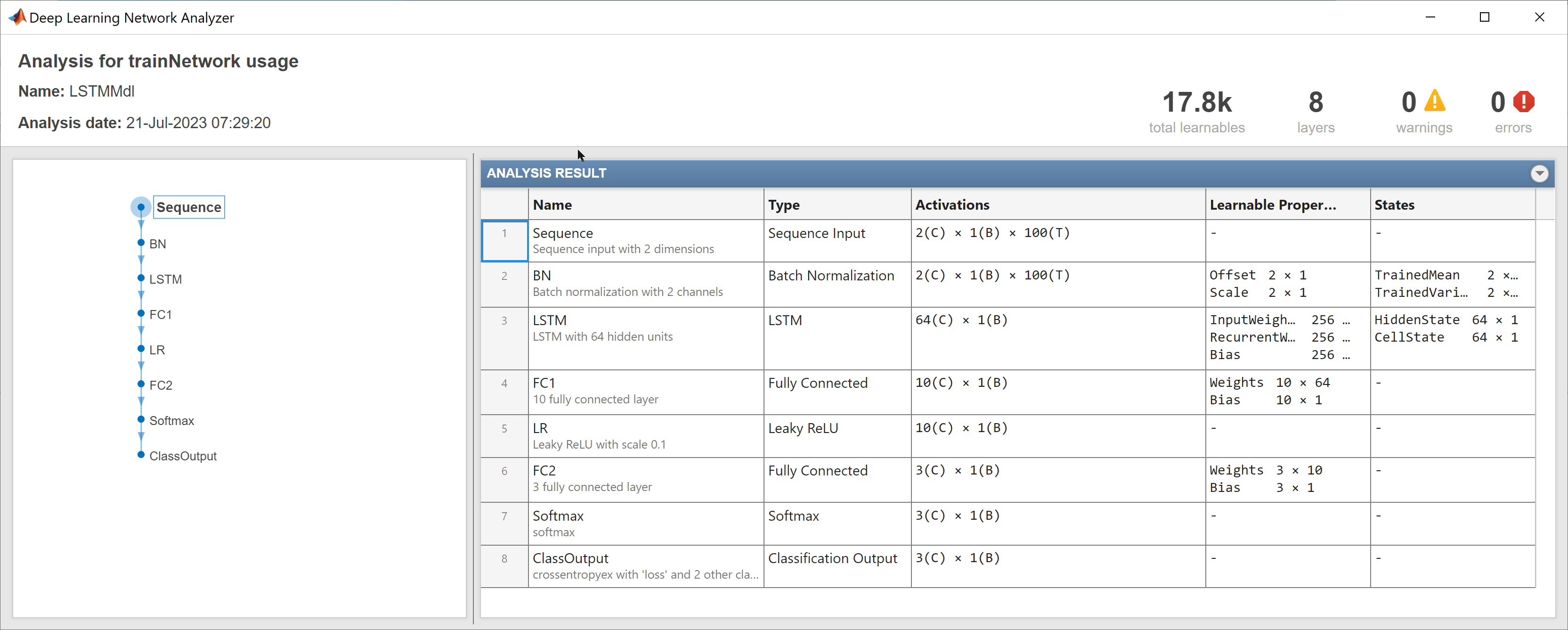
    Shuffle="every-epoch");

To train and validate the LSTM neural networks, set trainLSTM to true. Otherwise, this example loads the pretrained LSTM neural networks LSTMMdl and RiskyLSTMMdl in the MAT-file PretrainedLOBLSTMLvl3.mat, which is included with the Financial Toolbox documentation. Analyze the trained risky model.

trainLSTM = false;
if trainLSTM
    rng(1,"twister")
    LSTMMdl = trainnet(XT,yT,layersLSTM,"crossentropy",options);
    RiskyLSTMMdl = trainnet(XT,yT,layersLSTM,lossFcn,options);
else
    load PretrainedLOBLSTMLvl3
end
analyzeNetwork(RiskyLSTMMdl)

Assess Trained LSTM Model Quality

For each trained LSTM model, compute the model accuracy on the validation data and plot a confusion chart by following this procedure:

Predict responses and classification scores for the validation data by passing the feature validation data and the trained LSTM model to classify.
Pass the observed and predicted responses to confusionchart. Add column and row summaries to the chart.

[predScoresLSTM] = minibatchpredict(LSTMMdl,XV,InputDataFormats="CTB");
predYLSTM = scores2label(predScoresLSTM,classes);
accV = 100*mean(predYLSTM == yV)

accV = 91.0626

figure
cm = confusionchart(yV,predYLSTM);
cm.NormalizedValues;
cm.RowSummary = "row-normalized";
cm.ColumnSummary = "column-normalized";
cm.Title = "LSTM";

The conservative LSTM neural network predicts into the constant class for all validation observations. The 91% accuracy comes for free because this model acts like the naive model discussed in Engineer Features and Prepare Response Variable, which only ever predicts into the constant class. Such a model does not make money.

[predScoresRLSTM] = minibatchpredict(RiskyLSTMMdl,XV,InputDataFormats="CTB");
predYRLSTM = scores2label(predScoresRLSTM,classes);
accRiskyV = 100*mean(predYRLSTM == yV)

accRiskyV = 60.8731

figure
cm = confusionchart(yV,predYRLSTM);
cm.NormalizedValues;
cm.RowSummary = "row-normalized";
cm.ColumnSummary = "column-normalized";
cm.Title = "Risky LSTM";

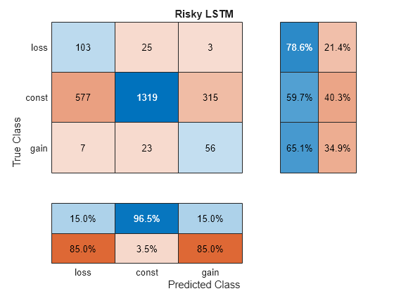
The risky LSTM model accuracy is about 61%. Despite this low value, the confusion chart suggests the following other aspects about the model's performance as it pertains to the trading strategy.

It correctly predicted about 65% of the 86 true gains, which makes money.
It correctly predicted about 79% of the 131 true losses, which prevents money loss.
It incorrectly predicted about 35% of the true gains as losses or constant, which results is a missed opportunity to make money.
It incorrectly predicted about 2% of the true losses as gains, which results in a money loss.

Plot ROC curves for both deep learning models.

rocLSTM = rocmetrics(yV,predScoresLSTM,classes);
rocRLSTM = rocmetrics(yV,predScoresRLSTM,classes);

figure
tiledlayout(1,2,TileSpacing="compact")
nexttile
plot(rocLSTM,ShowModelOperatingPoint=false)
title("ROC Curve: LSTM")
nexttile
plot(rocRLSTM,ShowModelOperatingPoint=false)
title("ROC Curve: Risky LSTM")

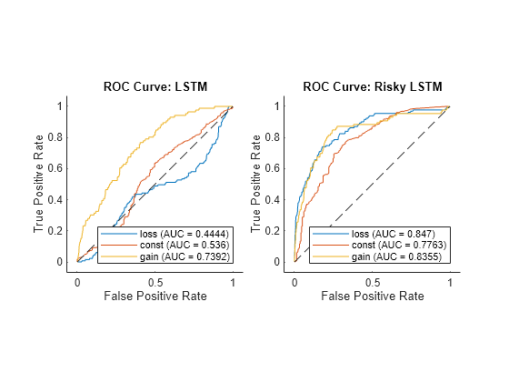
In general, each curve represents the ability of the model to distinguish observations that are in the corresponding class from the other two classes at various classification decision thresholds. For example, the blue curve corresponds to the ability of the classifiers to correctly distinguish losses from constants or gains. The diagonal dashed line is a hypothetical classifier that assigns observations into classes at random, which is a baseline for comparison. The curve of a good classifier increases very quickly and then levels off, making the area under the curve (AUC) close to 1. In other words, a good classifier has a high true positive rate for all classification decision thresholds, regardless of false positive rate levels produced. Note that the ROC curve does not consider false negative rates.

In this case, the risky LSTM is better at correctly distinguishing each class from the other two than the conservative LSTM; the AUCs of the risky LSTM are larger than the corresponding AUCs of the conservative LSTM.

Backtest Risky LSTM Model

Backtesting a predictive financial model dispatches it, and a trading strategy based on its predictions, on historical data. This action determines how well the model performs, with respect to the strategy. A backtest requires:

Historical data not used to train or validate the model (see Partition Data)
The target predictive model (The risky LSTM neural network RiskyLSTMMdl)
The model's predictions (signals) on the historical data
At least one trading strategy

Classify the forward price movements in the backtest data XBT using the risky LSTM neural network.

[predScoresRLSTMBT] = minibatchpredict(RiskyLSTMMdl,XBT,InputDataFormats="CTB");
predYRLSTMBT = scores2label(predScoresRLSTMBT,classes);

A trading strategy requires a way to predict outcomes and what financial decisions to make based on the outcomes. This example uses the following trading decision logic:

If the forward price direction is predicted to be a gain, invest all available money.
If the forward price direction is predicted to be a loss, cash out.
Otherwise, do nothing.

The rebalance function, located in this example in Local Functions, defines these predictive models:

Maximum Profit Model MaxProfit: A baseline model that perfectly predicts the next forward price direction, and therefore it always makes the right trading decisions.
Risky LSTM Neural Network RiskyLSTM: A model that predicts the next forward price direction by using the trained risky LSTM neural network RiskyLSTMMdl, with trading decisions based on its predictions.

The inputs of rebalance are:

Required asset weights w, which are the proportion of capital to invest across assets
Required asset prices p, which are not used in this example
Signal data s, optional data used to inform trading decisions
Optional user data structure to print backtest iteration information
Optional column of signal data to operate on for the strategy
Optional strategy name

Define the backtest strategies by passing the a function handle to rebalance to Create backtestStrategy. Set the following properties:

LookbackWindow=1, which indicates that the previous data point is available to the rebalance function during backtesting.
UserData=user_data, where user_data is a structure array containing the fields Counter, set initially to 0, and NumTestPoints, set to the backtest sample size.

Store the strategies in a vector.

user_data = struct("Counter",0,"NumTestPoints",nBT);
maxMoneyStrat = backtestStrategy("MaxProfit",@(w,p,s,u)rebalance(w,p,s,u,1,"MaxProfit"), ...
    LookbackWindow=1,UserData=user_data);
RiskyLSTMStrat = backtestStrategy("RiskyLSTM",@(w,p,s,u)rebalance(w,p,s,u,2,"RiskyLSTM"), ...
    LookbackWindow=1,UserData=user_data);
strategies = [maxMoneyStrat RiskyLSTMStrat];

strategies is a vector of backtestStrategy objects storing the backtest strategies.

Prepare the backtest engine by supplying the vector of backtestStrategy objects to backtestEngine.

bte = backtestEngine(strategies);

bte is a backtestEngine object specifying parameters for the backtest, including the risk-free rate RiskFreeRate, which is 0% by default.

Store the backtest forward price direction data and risky LSTM predictions in a timetable.

signalTT = timetable(yBT,predYRLSTMBT,RowTimes=tBT);

Store the backtest midprices in a timetable.

mpTT = timetable(mpBT,RowTimes=tBT);

Run the backtest by passing the backtest engine, midprice data, and signal data to runBacktest.

bte = runBacktest(bte,mpTT,signalTT);

Backtesting MaxProfit. Total progress: 5000 of 16190.
Backtesting MaxProfit. Total progress: 10000 of 16190.
Backtesting MaxProfit. Total progress: 15000 of 16190.
Backtesting RiskyLSTM. Total progress: 5000 of 16190.
Backtesting RiskyLSTM. Total progress: 10000 of 16190.
Backtesting RiskyLSTM. Total progress: 15000 of 16190.

bte is a backtestEngine object containing the results of the backtest.

Display a summary of the results by passing the completed backtest engine object to summary.

summary(bte)

ans=9×2 table
                       MaxProfit     RiskyLSTM 
                       __________    __________

    TotalReturn          0.076328      0.067524
    SharpeRatio           0.15212       0.13715
    Volatility         2.9873e-05    2.9433e-05
    AverageTurnover      0.010624     0.0090802
    MaxTurnover               0.5           0.5
    AverageReturn       4.544e-06    4.0366e-06
    MaxDrawdown        0.00018751    0.00055683
    AverageBuyCost              0             0
    AverageSellCost             0             0

The total nonannualized returns of the maximum profit and risky LSTM model are 7.6% and 6.8%, respectively. Therefore, the LSTM neural network performs well over the historical data.

Plot equity curves of the strategies by passing the completed backtest engine object to equityCurve.

figure
equityCurve(bte)

The equity curves indicate both strategies performed well, and are in close correspondence with each other.

Local Function

The rebalance function directs the backtest framework to perform the following trades:

When the model predicts a price gain, invest all available cash.
When the model predicts a price loss, cash out entirely.
When the model predicts a constant price, take no actions.

You can use this function only from in this script.

function [new_weights,user_data] = rebalance(weights,~,signalData,user_data,col,id)
    new_weights = weights;
    
    direction = signalData{:,col};
    if direction == "gain"
        new_weights = 1;    % Expect a gain --> Fully invest 
    end
    if direction == "loss"
        new_weights = 0;    % Expect loss --> Cash out, with risk-free rate of 0%
    end
    
    % Print iteration information at command line 
    user_data.Counter = user_data.Counter + 1;
    if (mod(user_data.Counter,5000) == 0)
        displayText = "Backtesting " + id + ". Total progress: " + num2str(user_data.Counter) + " of " + num2str(user_data.NumTestPoints) + ".";
        disp(displayText);
    end    
end

References

[1] Kolm, Petter, N., Jeremy Turiel, and Nicholas Westray. "Deep Order Flow Imbalance: Extracting Alpha at Multiple Horizons from the Limit Order Book." SSRN (August 2021): https://papers.ssrn.com/sol3/papers.cfm?abstract_id=3900141.

[2] LOBSTER Limit Order Book Data. Berlin: frischedaten UG (haftungsbeschränkt).

[3] NASDAQ Historical TotalView-ITCH Data. New York: The Nasdaq, Inc.

[4] Rubisov, Anton D. "Statistical Arbitrage Using Limit Order Book Imbalance." Master's thesis, University of Toronto, 2015.