creditexposures
Compute credit exposures from contract values
Syntax
Description
[
computes the counterparty credit exposures from an array of mark-to-market OTC
contract values. These exposures are used when calculating the CVA (credit value
adjustment) for a portfolio. exposures,exposurecpty]
= creditexposures(values,counterparties)
[
adds optional name-value arguments.exposures,exposurecpty]
= creditexposures(___,Name,Value)
[
computes the counterparty credit exposures from an array of mark-to-market OTC
contract values using optional name-value pair arguments for
exposures,exposurecpty,collateral]
= creditexposures(___,Name,Value)CollateralTable and Dates, the
collateral output is returned for the simulated
collateral amounts available to counterparties at each simulation date and over
each scenario.
Examples
After computing the mark-to-market contract values for a portfolio of swaps over many scenarios, compute the credit exposure for a particular counterparty. View the contract values and credit exposure over time.
First, load data (ccr.mat) containing the mark-to-market contract values for a portfolio of swaps over many scenarios.
load ccr.mat
% Look at one counterparty.
cpID = 4;
cpValues = squeeze(sum(values(:,swaps.Counterparty == cpID,:),2));
subplot(2,1,1)
simulationDates = datetime(simulationDates,"ConvertFrom","datenum");
plot(simulationDates,cpValues);
title(sprintf('Mark-to-Market Contract Values for Counterparty: %d',cpID));
xtickformat('MMMyy');
ylabel('Portfolio Value ($)')
% Compute the exposure by counterparty.
[exposures, expcpty] = creditexposures(values,swaps.Counterparty, ...
'NettingID',swaps.NettingID);
% View the credit exposure over time for the counterparty.
subplot(2,1,2)
cpIdx = find(expcpty == cpID);
plot(simulationDates,squeeze(exposures(:,cpIdx,:)));
title(sprintf('Exposure for Counterparty: %d',cpIdx));
xtickformat('MMMyy');
ylabel('Exposure ($)')
xlabel('Simulation Dates')

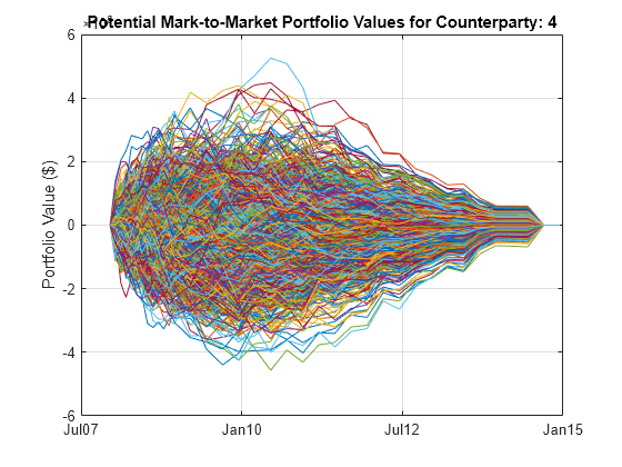
Load the data (ccr.mat) containing the mark-to-market contract values for a portfolio of swaps over many scenarios.
load ccr.matLook at one counterparty.
cpID = 4;
cpIdx = swaps.Counterparty == cpID;
cpValues = values(:,cpIdx,:);
simulationDates = datetime(simulationDates,"ConvertFrom","datenum");
plot(simulationDates,squeeze(sum(cpValues,2)));
grid on;
title(sprintf('Potential Mark-to-Market Portfolio Values for Counterparty: %d',cpID));
xtickformat('MMMyy');
ylabel('Portfolio Value ($)')

Compute the exposures.
netting = swaps.NettingID(cpIdx);
exposures = creditexposures(cpValues,cpID,'NettingID',netting);
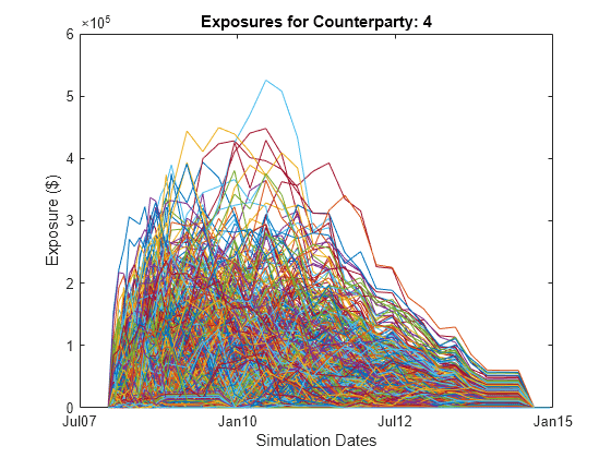
View the credit exposure over time for the counterparty.
figure;
plot(simulationDates,squeeze(exposures));
grid on
title(sprintf('Exposure for Counterparty: %d',cpID));
xtickformat('MMMyy');
ylabel('Exposure ($)')
xlabel('Simulation Dates')

Compute the credit exposure profiles.
simulationDates = convertTo(simulationDates,"datenum");
profilesBefore = exposureprofiles(simulationDates,exposures)
profilesBefore = struct with fields:
Dates: [37×1 double]
EE: [37×1 double]
PFE: [37×1 double]
MPFE: 2.1580e+05
EffEE: [37×1 double]
EPE: 2.8602e+04
EffEPE: 4.9579e+04
Consider a new trade with a counterparty. For this example, take another trade from the original swap portfolio and "copy" it for a new counterparty. This example is only for illustrative purposes.
newTradeIdx = 3;
newTradeValues = values(:,newTradeIdx,:);

% Append a new trade to your existing portfolio.
cpValues = [cpValues newTradeValues];
netting = [netting; cpID];
exposures = creditexposures(cpValues,cpID,'NettingID',netting);
Compute the new credit exposure profiles.
profilesAfter = exposureprofiles(simulationDates,exposures)
profilesAfter = struct with fields:
     Dates: [37×1 double]
        EE: [37×1 double]
       PFE: [37×1 double]
      MPFE: 2.4689e+05
     EffEE: [37×1 double]
       EPE: 3.1609e+04
    EffEPE: 5.6178e+04
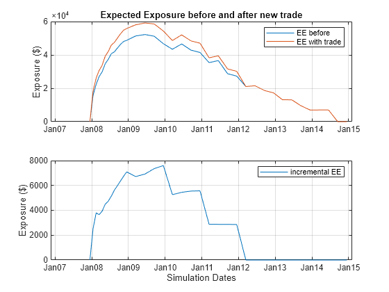
Visualize the expected exposures and the new trade's incremental exposure. Use the incremental exposure to compute the incremental credit value adjustment (CVA) charge.
figure;
subplot(2,1,1)
simulationDates = datetime(simulationDates,"ConvertFrom","datenum");
plot(simulationDates,profilesBefore.EE,...
    simulationDates,profilesAfter.EE);
grid on;
legend({'EE before','EE with trade'})
xtickformat('MMMyy');
title('Expected Exposure Before and After New Trade');
ylabel('Exposure ($)')

subplot(2,1,2)
incrementalEE = profilesAfter.EE - profilesBefore.EE;
plot(simulationDates,incrementalEE);
grid on;
legend('Incremental EE')
xtickformat('MMMyy');
ylabel('Exposure ($)')
xlabel('Simulation Dates')

Load the data (ccr.mat) containing the mark-to-market contract values for a portfolio of swaps over many scenarios.
load ccr.matOnly look at a single counterparty for this example.
cpID = 4;
cpIdx = swaps.Counterparty == cpID;
cpValues = values(:,cpIdx,:);
Compute the uncollateralized exposures.
exposures = creditexposures(cpValues,swaps.Counterparty(cpIdx),...
'NettingID',swaps.NettingID(cpIdx));
View the credit exposure over time for the counterparty.
simulationDates = datetime(simulationDates,"ConvertFrom","datenum");
plot(simulationDates,squeeze(exposures));
expYLim = get(gca,'YLim');
title(sprintf('Exposures for Counterparty: %d',cpID));
xtickformat('MMMyy');
ylabel('Exposure ($)')
xlabel('Simulation Dates')

Add a collateral agreement for the counterparty. The 'CollateralTable' parameter is a MATLAB® table. You can create tables from spreadsheets or other data sources, in addition to building them inline as seen here. For more information, see table.
collateralVariables = {'Counterparty';'PeriodOfRisk';'Threshold';'MinimumTransfer'};
periodOfRisk = 14;
threshold = 100000;
minTransfer = 10000;
collateralTable = table(cpID,periodOfRisk,threshold,minTransfer,...
'VariableNames',collateralVariables)collateralTable=1×4 table
Counterparty PeriodOfRisk Threshold MinimumTransfer
____________ ____________ _________ _______________
4 14 1e+05 10000
Compute the collateralized exposures.
[collatExp, collatcpty, collateral] = creditexposures(cpValues,...
    swaps.Counterparty(cpIdx),'NettingID',swaps.NettingID(cpIdx),...
    'CollateralTable',collateralTable,'Dates',simulationDates);
Plot the collateral levels and collateralized exposures.
figure;
subplot(2,1,1)
plot(simulationDates,squeeze(collateral));
set(gca,'YLim',expYLim);
title(sprintf('Collateral for Counterparty: %d',cpID));
xtickformat('MMMyy');
ylabel('Collateral ($)')
xlabel('Simulation Dates')

subplot(2,1,2)
plot(simulationDates,squeeze(collatExp));
set(gca,'YLim',expYLim);
title(sprintf('Collateralized Exposure for Counterparty: %d',cpID));
xtickformat('MMMyy');
ylabel('Exposure ($)')
xlabel('Simulation Dates');

Input Arguments
3-D array of simulated mark-to-market values of a portfolio of contracts
simulated over a series of simulation dates and across many scenarios,
specified as a
NumDates-by-NumContracts-by-NumScenarios
“cube” of contract values. Each row represents a different
simulation date, each column a different contract, and each
“page” is a different scenario from a Monte-Carlo simulation.
Data Types: double
Counterparties corresponding to each contract in
values, specified as a
NumContracts-element vector of counterparties.
Counterparties can be a vector of numeric IDs or a cell array of
counterparty names. By default, each counterparty is assumed to have one
netting set that covers all of its contracts. If counterparties are covered
by multiple netting sets, then use the NettingID
parameter. A value of NaN (or '' in a
cell array) indicates that a contract is not included in any netting set
unless otherwise specified by NettingID.
counterparties is case insensitive and leading or
trailing white spaces are removed.
Data Types: double | cell
Name-Value Arguments
Specify optional pairs of arguments as
Name1=Value1,...,NameN=ValueN, where Name is
the argument name and Value is the corresponding value.
Name-value arguments must appear after other arguments, but the order of the
pairs does not matter.
Before R2021a, use commas to separate each name and value, and enclose
Name in quotes.
Example: [exposures,exposurecpty] =
creditexposures(values,counterparties,'NettingID','10','ExposureType','Additive')
Netting set IDs to indicate to which netting set each contract in
values belongs, specified by a
NumContracts-element vector of netting set IDs.
NettingID can be a vector of numeric IDs or else
a cell array of character vector identifiers. The
creditexposures function uses
counterparties and NettingID
to define each unique netting set (all contracts in a netting set must
be with the same counterparty). By default, each counterparty has a
single netting set which covers all of their contracts. A value of
NaN (or '' in a cell array)
indicates that a contract is not included in any netting set.
NettingID is case insensitive and leading or
trailing white spaces are removed.
Data Types: double | cell
Calculation method for exposures, specified with values:
'Counterparty'— Compute exposures per counterparty.'Additive'— Compute additive exposures at the contract level. Exposures are computed per contract and sum to the total counterparty exposure.
Data Types: char
Table containing information on collateral agreements of counterparties, specified as a MATLAB table. The table consists of one entry (row) per collateralized counterparty and must have the following variables (columns):
'Counterparty'— Counterparty name or ID. The Counterparty name or ID should match the parameter'Counterparty'for theExposureTypeargument.'PeriodOfRisk'— Margin period of risk in days. The number of days from a margin call until the posted collateral is available from the counterparty.'Threshold'— Collateral threshold. When counterparty exposures exceed this amount, the counterparty must post collateral.'MinimumTransfer'— Minimum transfer amount. The minimum amount over/under the threshold required to trigger transfer of collateral.
Note
When computing collateralized exposures, both the
CollateralTable parameter and the
Dates parameter must be specified.
Data Types: table
Simulation dates corresponding to each row of the
values array, specified as a
NUMDATES-by-1 vector of
simulation dates. Dates is either a vector of
MATLAB date numbers or else a cell array of character vectors in
a known date format.
Note
When computing collateralized exposures, both the
CollateralTable parameter and the
Dates parameter must be specified.
Data Types: double | cell
Output Arguments
3-D array of credit exposures representing the potential losses from each
counterparty or contract at each date and over all scenarios. The size of
exposures depends on the
ExposureType input argument:
When
ExposureTypeis'Counterparty',exposuresreturns aNumDates-by-NumCounterparties-by-NumScenarios“cube” of credit exposures representing potential losses that could be incurred over all dates, counterparties, and scenarios, if a counterparty defaulted (ignoring any post-default recovery).When
ExposureTypeis'Additive',exposuresreturns aNumDates-by-NumContracts-by-NumScenarios“cube,” where each element is the additive exposure of each contract (over all dates and scenarios). Additive exposures sum to the counterparty-level exposure.
Counterparties that correspond to columns of the
exposures array, returned as
NumCounterparties or NumContracts
elements depending on the ExposureType.
Simulated collateral amounts available to counterparties at each
simulation date and over each scenario, returned as a
NumDates-by-NumCounterparties-by-NumScenarios
3D array. Collateral amounts are calculated using a Brownian bridge to
estimate contract values between simulation dates. For more information, see
Brownian Bridge. If the
CollateralTable was not specified, this output is
empty.
More About
Counterparty credit exposure refers to the risk that a counterparty in a financial transaction may default on its obligations, leading to potential financial losses for the other party involved in the transaction.
A Brownian bridge is used to simulate portfolio values at intermediate dates to compute collateral available at the subsequent simulation dates.
For example, to estimate collateral available at a particular simulation date, ti, you need to know the state of the portfolio at time ti – dt, where dt is the margin period of risk. Portfolio values are simulated at these intermediate dates by drawing from a distribution defined by the Brownian bridge between ti and the previous simulation date, ti–1.
If the contract values at time ti –1 and ti are known and you want to estimate the contract value at time tc (where tc is ti – dt), then a sample from a normal distribution is used with variance:
and with mean that is simply the linear interpolation of the contract values between the two simulation dates at time tc. For more details, see References.
References
[1] Lomibao, D., and S. Zhu. “A Conditional Valuation Approach for Path-Dependent Instruments.” August 2005.
[2] Pykhtin M. “Modeling credit exposure for collateralized counterparties.” December 2009.
[3] Pykhtin M., and S. Zhu. “A Guide to Modeling Counterparty Credit Risk.” GARP, July/August 2007, issue 37.
[4] Pykhtin, Michael., and Dan Rosen. “Pricing Counterparty Risk at the Trade Level and CVA Allocations.” FEDS Working Paper No. 10., February 1, 2010.
Version History
Introduced in R2014a
See Also
Topics
- Counterparty Credit Risk and CVA (Financial Instruments Toolbox)
- Wrong Way Risk with Copulas (Financial Instruments Toolbox)
MATLAB Command
You clicked a link that corresponds to this MATLAB command:
Run the command by entering it in the MATLAB Command Window. Web browsers do not support MATLAB commands.
Select a Web Site
Choose a web site to get translated content where available and see local events and offers. Based on your location, we recommend that you select: .
You can also select a web site from the following list
How to Get Best Site Performance
Select the China site (in Chinese or English) for best site performance. Other MathWorks country sites are not optimized for visits from your location.
Americas
- América Latina (Español)
- Canada (English)
- United States (English)
Europe
- Belgium (English)
- Denmark (English)
- Deutschland (Deutsch)
- España (Español)
- Finland (English)
- France (Français)
- Ireland (English)
- Italia (Italiano)
- Luxembourg (English)
- Netherlands (English)
- Norway (English)
- Österreich (Deutsch)
- Portugal (English)
- Sweden (English)
- Switzerland
- United Kingdom (English)