affineOutputView
Create output view for warping images
Syntax
Description
Examples
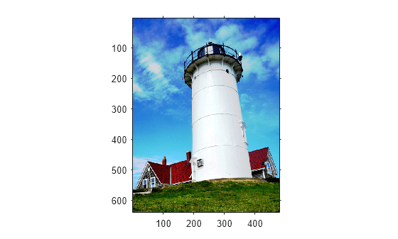
Read and display an image. To see the spatial extents of the image, make the axes visible.
I = imread("lighthouse.png");
iptsetpref(ImshowAxesVisible="on")
imshow(I)
Create a 2-D similarity transformation that resizes the image by a scale factor of 1.5 and rotates the image by 10 degrees.
tform = simtform2d(1.5,10,[0 0]);
Create an output view and specify that the input size is equal to the size of the input image. Also specify the "FollowOutput" bounds style.
szEqual = size(I);
viewEqual = affineOutputView(szEqual,tform,BoundsStyle="FollowOutput");
Apply the transformation to the input image using the first output view, then display the resulting image using spatial referencing information. Because the output view uses the "FollowOutput" bounds style, the transformation returns the complete transformed image. The extent of the output image is greater than the extent of the input image.
JEqual = imwarp(I,tform,OutputView=viewEqual);
imshow(JEqual,viewEqual)
title("Output View Using Full Image Size")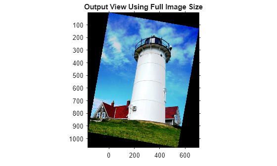
Create a second output view and specify a fixed input size that is smaller than the size of the input image.
szFixed = [200 300];
viewFixed = affineOutputView(szFixed,tform,BoundsStyle="FollowOutput");
Apply the transformation to the input image using the second output view, then display the resulting image using spatial referencing information. Although the output view uses the "FollowOutput" bounds style, the transformation does not return the complete transformed image. Instead, the transformation calculates what the image extent should be for a 200-by-300 pixel input, and crops the transformed image to fit the calculated image extent.
JFixed = imwarp(I,tform,OutputView=viewFixed);
imshow(JFixed,viewFixed)
title("Output View Using Fixed Image Size")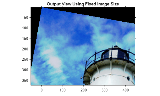
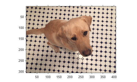
iptsetpref(ImshowAxesVisible="off")Read and display an image. To see the spatial extents of the image, make the axes visible.
I = imread("kobi.png");
I = imresize(I,0.25);
iptsetpref(ImshowAxesVisible="on")
imshow(I)

Create a 2-D affine transformation that shears the image in the horizontal direction. The amount of horizontal shear is equal to half of the height of the image.
A = [1 -0.5 0; 0 1 0; 0 0 1];
tform = affinetform2d(A);
Create three different output views for the image and transformation, using the three different bounds styles.
szI = size(I);
followOutput = affineOutputView(szI,tform,BoundsStyle="FollowOutput");
centerOutput = affineOutputView(szI,tform,BoundsStyle="CenterOutput");
sameAsInput  = affineOutputView(szI,tform,BoundsStyle="SameAsInput");
Apply the transformation to the input image using each of the different output view styles. Then, display the resulting images using the spatial referencing information returned by the affineOutputView function.
The "FollowOutput" bounds style returns the complete transformed image. The transformed image is wider than the original image.
JFollowOutput = imwarp(I,tform,OutputView=followOutput);
imshow(JFollowOutput,followOutput)
title("FollowOutput Bounds Style")
The "CenterOutput" bounds style crops the transformed image to the size of the input image. The crop window is centered on the transformed image, so the top-left corner of the crop window is not at the origin.
BCenterOutput = imwarp(I,tform,OutputView=centerOutput);
imshow(BCenterOutput,centerOutput)
title("CenterOutput Bounds Style")
The "SameAsInput" bounds style also crops the transformed image to the size of the input image. The top-left corner of the crop window is at the origin.
BSameAsInput  = imwarp(I,tform,OutputView=sameAsInput);
imshow(BSameAsInput,sameAsInput)
title("SameAsInput Bounds Style")
iptsetpref(ImshowAxesVisible="off")Read and display an image. To see the spatial extents of the image, make the axes visible.
I = imread("kobi.png");
I = imresize(I,0.25);
iptsetpref(ImshowAxesVisible="on")
imshow(I)
Get the size of the image.
szI = size(I);
View for Transformation Without Translation
Create a 2-D affine transformation that consists only of horizontal shear.
S = [1 -0.5 0; 0 1 0; 0 0 1];
tformShear = affinetform2d(S);
Create an output view for the shear transformation.
refShear = affineOutputView(szI,tformShear);
Apply the shear-only transformation to the input image. Then, display the resulting image using the spatial referencing information. By default, the output view crops the transformed image to the size of the input image. Because the transformation does not include translation, the crop window is centered on the transformed image.
JShear = imwarp(I,tformShear,OutputView=refShear);
imshow(JShear,refShear)
title("Shearing Only")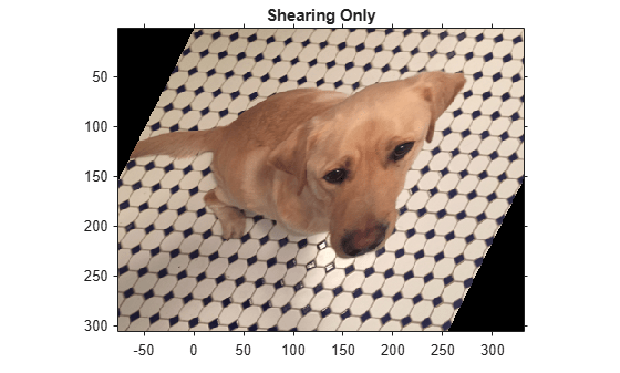
Views for Transformation With Translation
Create a 2-D affine transformation that includes the same amount of horizontal shear as tformShear. Add horizontal translation by amount tx, and vertical translation by amount ty.
tx = 100;
ty = 50;
T = S + [0 0 tx; 0 0 ty; 0 0 0];
tformTrans = affinetform2d(T);
Create an output view for the shear-and-translation transformation. Use the default bounds style, which is centered on the output image (ignoring the effect of translation).
refTrans = affineOutputView(szI,tformTrans);
Apply the shear-and-translation transformation to the input image. Then, display the resulting image using the spatial referencing information. Again, the output view crops the transformed image to the size of the input image. However, because the transformation includes translation, the crop window is not centered on the transformed image.
JTrans = imwarp(I,tformTrans,OutputView=refTrans);
imshow(JTrans,refTrans)
title("Shearing With Translation")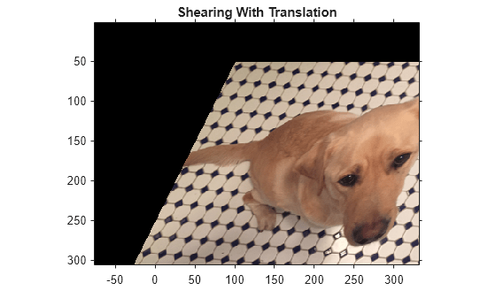
For comparison, create an output view for the shear-and-translation transformation that uses the "FollowOutput" bounds style.
refFollowOutput = affineOutputView(szI,tformTrans,BoundsStyle="FollowOutput");Apply the shear-and-translation transformation to the input image. Then, display the resulting image using the spatial referencing information. Because the bounds style is "FollowOutput", the output view considers the effect of translation, and the crop window is centered on the transformed image.
JTrans = imwarp(I,tformTrans,OutputView=refFollowOutput);
imshow(JTrans,refFollowOutput)
title("Shearing With Translation and FollowOutput Bounds Style")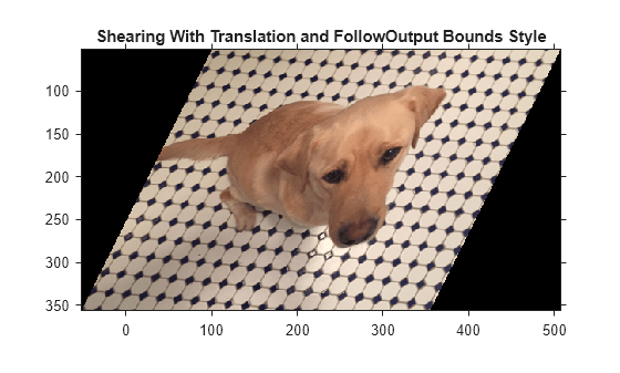
View for Transformation with Offset in Spatial Referencing
Define a spatial referencing object for an image of size szI. Shift the position of the image in world coordinates by adding an offset to the world limits.
xshift = 100;
yshift = 50;
xWorldLim = [xshift szI(2)+xshift];
yWorldLim = [yshift szI(1)+yshift];
refIn = imref2d(szI,xWorldLim,yWorldLim);
Create another output view for the shear-only transformation, specifying the input spatial referencing object.
refOut = affineOutputView(refIn,tformShear);
Apply the shear-only transformation to the input image. Then, display the resulting image using the output spatial referencing information. By default, the output view crops the transformed image to the size of the input image. Because the input spatial referencing includes translation of the image in world coordinates, the crop window is not centered on the transformed image.
JRef = imwarp(I,tformShear,OutputView=refOut);
imshow(JRef,refOut)
title("Shearing with Input Spatial Referencing")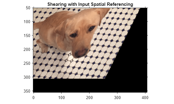
iptsetpref(ImshowAxesVisible="off")Input Arguments
Output Arguments
Algorithms
affineOutputView determines the spatial extent of
the output spatial referencing object by mapping locations in the output image to the
corresponding locations in the input image, using the intrinsic coordinate system (an inverse
mapping). The mapping ignores translation in the transformation and offsets of the image in an
input spatial referencing system. For more information, see Image Coordinate Systems.