Main Content

bwboundaries

Trace object boundaries in binary image

Description

B = bwboundaries(BW) traces the exterior boundaries of objects, as well as boundaries of holes inside these objects, in the binary image BW. bwboundaries also traces the exterior and hole boundaries of children objects completely enclosed by parent objects. The function returns B, a cell array of boundary pixel locations.

The figure illustrates these components.
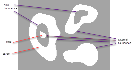
Parent objects in a binary image are white blobs that can have holes. Children objects appear as islands within the holes.

example

B = bwboundaries(BW,conn) specifies the connectivity conn to use when tracing object boundaries.

B = bwboundaries(___,options) traces the exterior boundaries of objects and specifies whether you want to include the boundaries of holes by setting options as either "holes" or "noholes".

example

B = bwboundaries(___,Name=Value) specifies the trace style and the order of returned vertex coordinates using name-value arguments (since R2023a).

[B,L] = bwboundaries(___) also returns a label matrix L that labels the objects and holes.

example

[B,L,n,A] = bwboundaries(___) also returns n, the number of objects found, and A, an adjacency matrix.

example

Examples

collapse all

Read grayscale image into the workspace.

I = imread('rice.png');

Convert grayscale image to binary image using local adaptive thresholding.

BW = imbinarize(I);

Calculate boundaries of regions in image and overlay the boundaries on the image.

[B,L] = bwboundaries(BW,'noholes');
imshow(label2rgb(L, @jet, [.5 .5 .5]))
hold on
for k = 1:length(B)
   boundary = B{k};
   plot(boundary(:,2), boundary(:,1), 'w', 'LineWidth', 2)
end

Figure contains an axes object. The hidden axes object contains 152 objects of type image, line.

Read binary image into the workspace.

BW = imread('blobs.png');

Calculate boundaries of regions in the image.

[B,L,N,A] = bwboundaries(BW);

Display the image with the boundaries overlaid. Add the region number next to every boundary (based on the label matrix). Use the zoom tool to read individual labels.

imshow(BW); hold on;
colors=['b' 'g' 'r' 'c' 'm' 'y'];
for k=1:length(B),
  boundary = B{k};
  cidx = mod(k,length(colors))+1;
  plot(boundary(:,2), boundary(:,1),...
       colors(cidx),'LineWidth',2);

  %randomize text position for better visibility
  rndRow = ceil(length(boundary)/(mod(rand*k,7)+1));
  col = boundary(rndRow,2); row = boundary(rndRow,1);
  h = text(col+1, row-1, num2str(L(row,col)));
  set(h,'Color',colors(cidx),'FontSize',14,'FontWeight','bold');
end

Figure contains an axes object. The hidden axes object contains 79 objects of type image, line, text.

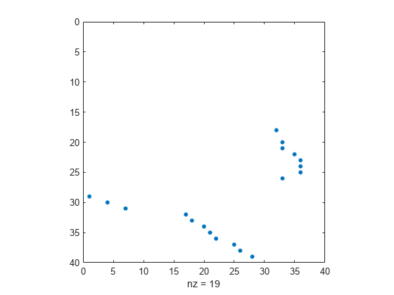
Display the adjacency matrix using the spy function.

figure
spy(A);

Figure contains an axes object. The axes object with xlabel nz = 19 contains a line object which displays its values using only markers.

Read binary image into workspace.

BW = imread('blobs.png');

Calculate boundaries.

[B,L,N] = bwboundaries(BW);

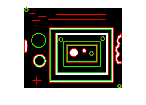
Display object boundaries in red and hole boundaries in green.

imshow(BW); hold on;
for k=1:length(B),
   boundary = B{k};
   if(k > N)
     plot(boundary(:,2), boundary(:,1), 'g','LineWidth',2);
   else
     plot(boundary(:,2), boundary(:,1), 'r','LineWidth',2);
   end
end

Figure contains an axes object. The hidden axes object contains 40 objects of type image, line.

Read image into workspace.

BW = imread('blobs.png');

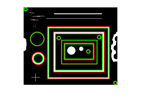
Display parent boundaries in red and their holes in green.

[B,L,N,A] = bwboundaries(BW); 
figure; imshow(BW); hold on; 
% Loop through object boundaries  
for k = 1:N 
    % Boundary k is the parent of a hole if the k-th column 
    % of the adjacency matrix A contains a non-zero element 
    if (nnz(A(:,k)) > 0) 
        boundary = B{k}; 
        plot(boundary(:,2),... 
            boundary(:,1),'r','LineWidth',2); 
        % Loop through the children of boundary k 
        for l = find(A(:,k))' 
            boundary = B{l}; 
            plot(boundary(:,2),... 
                boundary(:,1),'g','LineWidth',2); 
        end 
    end 
end

Figure contains an axes object. The hidden axes object contains 23 objects of type image, line.

Input Arguments

collapse all

Binary image, specified as a 2-D logical or numeric matrix. For numeric input, any nonzero pixels are considered to be 1 (true).

Data Types: single | double | int8 | int16 | int32 | int64 | uint8 | uint16 | uint32 | uint64 | logical

Pixel connectivity, specified as one of the values in this table.

Value

Meaning

Two-Dimensional Connectivities

4

Pixels are connected if their edges touch. Two adjoining pixels are part of the same object if they are both on and are connected along the horizontal or vertical direction.

Center pixel connected to four pixels

Current pixel is shown in gray.

8

Pixels are connected if their edges or corners touch. Two adjoining pixels are part of the same object if they are both on and are connected along the horizontal, vertical, or diagonal direction.

Center pixel connected to eight pixels

Current pixel is shown in gray.

Data Types: double

Determine whether to search for both parent and child boundaries, specified as either of the following:

Option

Meaning

"holes"

Search for both object and hole boundaries. This is the default.

"noholes"

Search only for object (parent and child) boundaries. This can provide better performance.

Data Types: char | string

Name-Value Arguments

Specify optional pairs of arguments as Name1=Value1,...,NameN=ValueN, where Name is the argument name and Value is the corresponding value. Name-value arguments must appear after other arguments, but the order of the pairs does not matter.

Example: B = bwboundaries(BW,TraceStyle="pixeledge") traces the boundary of objects in binary image BW along the outer edge of boundary pixels.

Since R2023a

Trace style along the boundary, specified as "pixelcenter" or "pixeledge".

Trace Style

Meaning

"pixelcenter"

Trace the boundary as a polygon connecting the centers of the boundary pixels.

"pixeledge"

Trace the boundary as a polygon along the outer edge of the boundary pixels.

Since R2023a

Order of the returned vertex coordinates, specified as "yx" or "xy".

Trace Style

Meaning

"yx"

Return boundary vertices as (y, x) coordinates, which is the same order as (row, column) coordinates

"xy"

Return boundary vertices as (x, y) coordinates

Output Arguments

collapse all

Coordinates of the boundary vertices, returned as a p-by-1 cell array, where p is the number of objects and holes. The first n cells in B are object boundaries and the remaining cells are hole boundaries.

Each cell in the cell array contains a q-by-2 matrix. Each row in the matrix contains the coordinates of a vertex along the boundary. q is the number of boundary vertices for the corresponding region.

Label matrix of contiguous regions, returned as a 2-D matrix of nonnegative integers. The kth region includes all elements in L that have value k. The number of objects and holes represented by L is equal to max(L(:)). The zero-valued elements of L make up the background.

Data Types: double

Number of objects found, returned as a nonnegative integer.

Data Types: double

Parent-child dependencies between boundaries and holes, returned as a square, sparse, logical matrix with side of length max(L(:)). The rows and columns of A correspond to the positions of boundaries stored in B. A(i,j)=1 means that object i is a child of object j. The boundaries that enclose or are enclosed by the k-th boundary can be found using A as follows:

enclosing_boundary  = find(A(k,:));
enclosed_boundaries = find(A(:,k));

Data Types: double

Algorithms

The bwboundaries function implements the Moore-Neighbor tracing algorithm modified by Jacob's stopping criteria. This function is based on the boundaries function presented in the first edition of Digital Image Processing Using MATLAB [1].

References

[1] Gonzalez, R. C., R. E. Woods, and S. L. Eddins, Digital Image Processing Using MATLAB, New Jersey, Pearson Prentice Hall, 2004.

Extended Capabilities

Version History

Introduced before R2006a

expand all

Go to top of page