polyval

R2026b

Polynomial evaluation

Syntax

y = polyval(coeffs,x)

[y,delta] = polyval(coeffs,x,fitStats)

y = polyval(coeffs,x,[],centerScale)

[y,delta] = polyval(coeffs,x,fitStats,centerScale)

Description

y = polyval(coeffs,x) evaluates the polynomial defined by the coefficient vector coeffs at each point in x. The vector coeffs has length n+1 and contains the coefficients of an nth-degree polynomial p in descending powers:

$$p(x)=\mathrm{coeffs}(1)\cdot x^n+\mathrm{coeffs}(2)\cdot x^{n-1}+\mathrm{...}+\mathrm{coeffs}(n)\cdot x+\mathrm{coeffs}(n+1).$$

The polynomial coefficients in coeffs can be calculated for different purposes by functions like polyint, polyder, and polyfit, but you can specify any vector for the coefficients.

To evaluate a polynomial in a matrix sense, use polyvalm instead.

[y,delta] = polyval(coeffs,x,fitStats) uses the optional output structure fitStats produced by polyfit to generate error estimates. delta is an estimate of the standard error in predicting a future observation at x by coeffs(x).

y = polyval(coeffs,x,[],centerScale) or [y,delta] = polyval(coeffs,x,fitStats,centerScale) evaluates the polynomial at the normalized points $$\frac{x-centerScale(1)}{centerScale(2)}$$, where centerScale is produced by polyfit. Use the second syntax to evaluate a fitted polynomial and compute error estimates, with coefficients, fit statistics, and normalization parameters obtained from polyfit.

Examples

Evaluate Polynomial at Several Points

Evaluate the polynomial $p\left(x\right)=3x^2+2x+1$ at the points $x=5,7,9$. The polynomial coefficients can be represented by the vector [3 2 1].

coeffs = [3 2 1];
x = [5 7 9];
y = polyval(coeffs,x)

y = 1×3

    86   162   262

Integrate Quartic Polynomial

Evaluate the definite integral

$$I={\int }_{-1}^3\left(3x^4-4x^2+10x-25\right)dx.$$

Create a vector to represent the polynomial integrand $$3x^4-4x^2+10x-25$$. The $x^3$ term is absent and thus has a coefficient of 0.

coeffs = [3 0 -4 10 -25];

Use polyint to integrate the polynomial using a constant of integration equal to 0.

q = polyint(coeffs)

q = 1×6

    0.6000         0   -1.3333    5.0000  -25.0000         0

Find the value of the integral by evaluating q at the limits of integration.

a = -1;
b = 3;
I = diff(polyval(q,[a b]))

I = 
49.0667

Linear Regression with Error Estimate

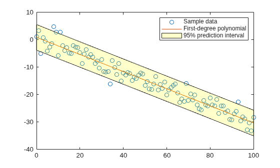
Fit a linear model to a set of data points and plot the results, including an estimate of a 95% prediction interval.

Create a few vectors of sample data points (x, y). Use polyfit to fit a first-degree polynomial to the data. Specify two outputs to return the coefficients for the linear fit as well as the error estimation structure.

x = 0:100; 
y = -0.3*x + 2*randn(1,101); 
[coeffs,fitStats] = polyfit(x,y,1);

Evaluate the first-degree polynomial at the points in x. Specify the error estimation structure as the third input so that polyval calculates an estimate of the standard error. The standard error estimate is returned in delta.

[yfit,delta] = polyval(coeffs,x,fitStats);

Plot the original data, linear fit, and 95% prediction interval $yfit\pm 2\Delta$.

plot(x,y,"o")
hold on
plot(x,yfit)

xinterval = [x flip(x)];
yinterval = [yfit-2*delta flip(yfit)+2*delta];
interval = fill(xinterval,yinterval,"yellow",FaceAlpha=0.2);

legend("Sample data","First-degree polynomial","95% prediction interval")
hold off

Normalize Data to Improve Numerical Conditioning

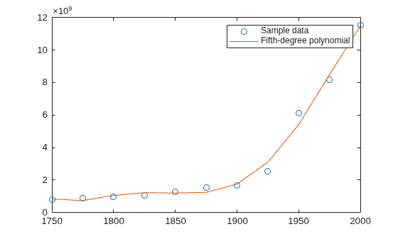
Create sample population data for the years 1750 - 2000 and plot the data points.

x = 1750:25:2000;
y = 1e6*[791 856 978 1050 1262 1544 1650 2532 6122 8170 11560];

Use polyfit to fit a fifth-degree polynomial to the data. You can improve numerical conditioning by normalizing the query vector before fitting a polynomial. This example normalizes the year data and computes a fifth-degree polynomial fit. The function also returns the center and scale used for normalization.

[coeffsNorm,~,centerScale] = polyfit(x,y,5,Normalize=true);

Normalize the query points to the same center and scale, and then evaluate the polynomial by specifying centerScale when calling the polyval function. Then, plot the results.

yfit = polyval(coeffsNorm,x,[],centerScale);

plot(x,y,"o")
hold on
plot(x,yfit)
legend("Sample data","Fifth-degree polynomial")
hold off

Input Arguments

coeffs — Polynomial coefficients

vector

Polynomial coefficients, specified as a vector. coeffs has length n+1 and contains the polynomial coefficients in descending powers, where the polynomial degree is n. For example, the vector [1 0 1] represents the polynomial $$x^2+1$$.

The polynomial coefficients in coeffs can be calculated by functions like polyint, polyder, and polyfit, but you can specify any vector for the coefficients. For more information, see Create and Evaluate Polynomials.

Data Types: double | single
Complex Number Support: Yes

x — Query points

vector

Query points, specified as a vector. polyval evaluates the polynomial coeffs at the points in x and returns the corresponding function values in y.

Data Types: double | single
Complex Number Support: Yes

fitStats — Fit statistics

structure

Fit statistics, specified as a structure returned by polyfit. The fitStats structure must contain these fields.

Field	Description
R	Triangular R factor (possibly permuted) from a QR decomposition of the Vandermonde matrix of x
df	Degrees of freedom of the fit
normr	Euclidean norm of the residuals
rsquared (since R2024a)	Coefficient of determination (unadjusted R-squared)

centerScale — Center and scaling values

two-element vector

Center and scaling values used to normalize the query points in x before evaluating the polynomial, specified as a two-element vector.

If you use polyfit with Normalize=true to compute the polynomial coefficients, then specify centerScale when calling polyval to normalize the query points to the same center and scale.

Output Arguments

y — Function values

vector

Function values, returned as a vector of the same size as the query points x. The vector contains the result of evaluating the polynomial coeffs at each point in x.

delta — Standard error for prediction

vector

Standard error for prediction, returned as a vector of the same size as the query points x.

Generally, an interval of y ± Δ corresponds to a roughly 68% prediction interval for future observations of large samples, and y ± 2Δ a roughly 95% prediction interval.

If the coefficients in coeffs are least-squares estimates computed by polyfit, and the errors in the data input to polyfit are independent, normal, and have constant variance, then y ± Δ is at least a 50% prediction interval.

Extended Capabilities

Tall Arrays

Calculate with arrays that have more rows than fit in memory.

The polyval function supports tall arrays with the following usage notes and limitations:

If x is a tall array, then it must be a column vector.

For more information, see Tall Arrays.

C/C++ Code Generation
Generate C and C++ code using MATLAB® Coder™.

GPU Code Generation
Generate CUDA® code for NVIDIA® GPUs using GPU Coder™.

Thread-Based Environment

Run code in the background using MATLAB® backgroundPool or accelerate code with Parallel Computing Toolbox™ ThreadPool.

The polyval function fully supports thread-based environments. For more information, see Run MATLAB Functions in Thread-Based Environment.

GPU Arrays

Accelerate code by running on a graphics processing unit (GPU) using Parallel Computing Toolbox™.

The polyval function fully supports GPU arrays. To run the function on a GPU, specify the input data as a gpuArray (Parallel Computing Toolbox). For more information, see Run MATLAB Functions on a GPU (Parallel Computing Toolbox).

Distributed Arrays

Partition large arrays across the combined memory of your cluster using Parallel Computing Toolbox™.

The polyval function fully supports distributed arrays. For more information, see Run MATLAB Functions with Distributed Arrays (Parallel Computing Toolbox).

Version History

Introduced before R2006a