polyfit

R2026b

Polynomial curve fitting

Syntax

coeffs = polyfit(x,y,n)

[coeffs,fitStats] = polyfit(x,y,n)

[coeffs,fitStats,centerScale] = polyfit(x,y,n,Normalize=tf)

Description

coeffs = polyfit(x,y,n) returns the coefficients for a polynomial p(x) of degree n that best fits the data in y in a least-squares sense, where the resulting polynomial is:

$$p(x)=\mathrm{coeffs}(1)\cdot x^n+\mathrm{coeffs}(2)\cdot x^{n-1}+\mathrm{...}+\mathrm{coeffs}(n)\cdot x+\mathrm{coeffs}(n+1).$$

[coeffs,fitStats] = polyfit(x,y,n) also returns fit statistics that can be used to estimate prediction error with the polyval function.

[coeffs,fitStats,centerScale] = polyfit(x,y,n,Normalize=tf) provides the option to apply normalization when fitting. If you set Normalize to true, polyfit centers x at 0 and scales it to have a standard deviation of 1 according to the transformation $$\widehat{x}=\frac{x-\overline{x}}{{\sigma }_x}.$$ In this case, polyfit also returns the centerScale output as a two-element vector that contains the center and scaling values, which are mean(x) and std(x). If you set Normalize to false, polyfit does not transform x, and centerScale is a two-element vector that contains 0 and 1. (since R2026b)

Before R2026b: Normalization is controlled implicitly by the number of output arguments. Returning a third output argument enables normalization automatically. See Version History for more information.

Examples

Simple Linear Regression

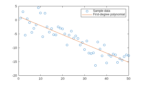
Fit a simple linear regression model to a set of discrete 2-D data points.

Create two vectors of sample data points (x, y). Fit a first-degree polynomial to the data.

x = 1:50; 
y = -0.3*x + 2*randn(1,50); 
coeffs = polyfit(x,y,1); 

Evaluate the fitted polynomial at the points in x. Plot the resulting linear regression model with the data.

f = polyval(coeffs,x);

plot(x,y,"o")
hold on
plot(x,f)
legend("Sample data","First-degree polynomial")
hold off

Fit Polynomial to Trigonometric Function

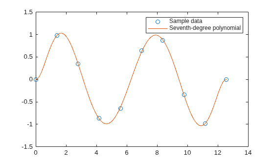
Generate 10 equally spaced points along a sine curve in the interval [0,4*pi].

x = linspace(0,4*pi,10);
y = sin(x);

Fit a seventh-degree polynomial to the data.

coeffs = polyfit(x,y,7);

Evaluate the fitted polynomial on a finer grid and plot the results.

x2 = linspace(0,4*pi);
yfit = polyval(coeffs,x2);

plot(x,y,"o")
hold on
plot(x2,yfit)
legend("Sample data","Seventh-degree polynomial")
hold off

Fit Polynomial to Set of Points

Create a vector of 5 equally spaced points in the interval [0,1], and evaluate $y\left(x\right)=\frac{1}{1+x}$ at those points.

x = linspace(0,1,5);
y = 1./(1+x);

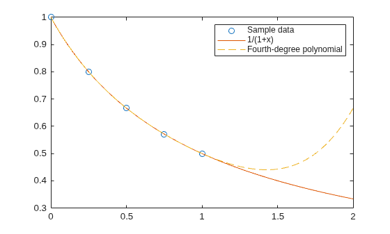
Fit a fourth-degree polynomial to the data. In general, for n points, you can fit a polynomial of degree n-1 to exactly pass through the points.

coeffs = polyfit(x,y,4);

Evaluate the original function and the polynomial fit on a finer grid of points between 0 and 2.

x2 = linspace(0,2);
yfcn = 1./(1+x2);
yfit = polyval(coeffs,x2);

Plot the function values and the polynomial fit in the wider interval [0,2], with the points used to obtain the polynomial fit highlighted as circles. The polynomial fit is good in the original [0,1] interval, but quickly diverges from the original function outside of that interval.

plot(x,y,"o")
hold on
plot(x2,yfcn)
plot(x2,yfit,"--")
legend("Sample data","1/(1+x)","Fourth-degree polynomial")
hold off

Fit Polynomial to Error Function

First generate a vector of equally spaced points in the interval [0,2.5], and then evaluate erf(x) at those points.

x = (0:0.1:2.5)';
y = erf(x);

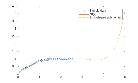
Fit a sixth-degree polynomial to the data.

coeffs = polyfit(x,y,6)

coeffs = 1×7

    0.0084   -0.0983    0.4217   -0.7435    0.1471    1.1064    0.0004

To see how good the fit is, evaluate the polynomial at the data points and generate a table showing the data, fit, and error.

yfit = polyval(coeffs,x);
T = table(x,y,yfit,y-yfit,VariableNames=["X" "Y" "Fit" "FitError"])

T = 26×4 table
     X        Y          Fit         FitError  
    ___    _______    __________    ___________

      0          0    0.00044117    -0.00044117
    0.1    0.11246       0.11185     0.00060836
    0.2     0.2227       0.22231     0.00039189
    0.3    0.32863       0.32872    -9.7429e-05
    0.4    0.42839        0.4288    -0.00040661
    0.5     0.5205       0.52093    -0.00042568
    0.6    0.60386       0.60408    -0.00022824
    0.7     0.6778       0.67775     4.6383e-05
    0.8     0.7421       0.74183     0.00026992
    0.9    0.79691       0.79654     0.00036515
      1     0.8427       0.84238      0.0003164
    1.1    0.88021       0.88005     0.00015948
    1.2    0.91031       0.91035    -3.9919e-05
    1.3    0.93401       0.93422      -0.000211
    1.4    0.95229       0.95258    -0.00029933
    1.5    0.96611       0.96639    -0.00028097
      ⋮

In this interval, the interpolated values and the actual values are fairly close. Create a plot to show that outside this interval, the extrapolated values quickly diverge from the actual data.

x2 = (0:0.1:5)';
fcnextrap = erf(x2);
fitextrap = polyval(coeffs,x2);

plot(x,y,"o")
hold on
plot(x2,fcnextrap)
plot(x2,fitextrap,"--")
xlim([0 5])
legend("Sample data","erf(x)","Sixth-degree polynomial")
hold off

Normalize Data to Improve Numerical Conditioning

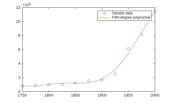
Create sample population data for the years 1750 - 2000 and plot the data points.

x = 1750:25:2000;
y = 1e6*[791 856 978 1050 1262 1544 1650 2532 6122 8170 11560];

Use polyfit to fit a fifth-degree polynomial to the data. You can improve numerical conditioning by normalizing the query vector before fitting a polynomial. This example normalizes the year data and computes a fifth-degree polynomial fit. The function also returns the center and scale used for normalization.

[coeffsNorm,~,centerScale] = polyfit(x,y,5,Normalize=true);

Normalize the query points to the same center and scale, and then evaluate the polynomial by specifying centerScale when calling the polyval function. Then, plot the results.

yfit = polyval(coeffsNorm,x,[],centerScale);

plot(x,y,"o")
hold on
plot(x,yfit)
legend("Sample data","Fifth-degree polynomial")
hold off

Linear Regression with Error Estimate

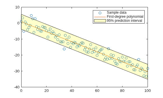
Fit a linear model to a set of data points and plot the results, including an estimate of a 95% prediction interval.

Create a few vectors of sample data points (x, y). Use polyfit to fit a first-degree polynomial to the data. Specify two outputs to return the coefficients for the linear fit as well as the error estimation structure.

x = 0:100; 
y = -0.3*x + 2*randn(1,101); 
[coeffs,fitStats] = polyfit(x,y,1);

Evaluate the first-degree polynomial at the points in x. Specify the error estimation structure as the third input so that polyval calculates an estimate of the standard error. The standard error estimate is returned in delta.

[yfit,delta] = polyval(coeffs,x,fitStats);

Plot the original data, linear fit, and 95% prediction interval $yfit\pm 2\Delta$.

plot(x,y,"o")
hold on
plot(x,yfit)

xinterval = [x flip(x)];
yinterval = [yfit-2*delta flip(yfit)+2*delta];
interval = fill(xinterval,yinterval,"yellow",FaceAlpha=0.2);

legend("Sample data","First-degree polynomial","95% prediction interval")
hold off

Input Arguments

x — Query points

vector

Query points, specified as a vector. The query points in x correspond to the fitted values in y. If x is not a vector, then polyfit converts it into a column vector x(:).

An ill-conditioned fit can result from repeated (or nearly repeated) query points, widely spaced query points, or using a high polynomial degree. To improve the conditioning, add distinct query points, normalize the data by specifying Normalize=true, or reduce the degree.

Data Types: double | single
Complex Number Support: Yes

y — Fitted values at query points

vector

Fitted values at query points, specified as a vector. The fitted values in y correspond to the query points in x. If y is not a vector, then polyfit converts it into a column vector y(:).

Data Types: double | single
Complex Number Support: Yes

n — Degree of polynomial fit

positive integer scalar

Degree of polynomial fit, specified as a positive integer scalar. n specifies the polynomial power of the first coefficient in coeffs.

An ill-conditioned fit can result from a high polynomial degree. To improve the conditioning, reduce the degree.

tf — Option to normalize query points

true or 1 | false or 0

Since R2026b

Option to normalize the query points in x before fitting, specified as one of these values for the Normalize parameter:

• true or 1 — Normalize the query points in x before fitting the polynomial by centering them at 0 and scaling them to a standard deviation of 1.

• false or 0 — Do not normalize the query points in x before fitting the polynomial.

If you specify the third output centerScale, then polyfit uses Normalize=true by default. Otherwise, the default is Normalize=false.

Normalization improves numerical conditioning, especially for higher-degree polynomials or widely spaced query points.

Example: [coeffs,~,centerScale] = polyfit(x,y,n,Normalize=true) normalizes the query points in x, fits a polynomial of degree n, and returns the center and scaling value in addition to the polynomial coefficients in terms of the normalized query points.

Output Arguments

coeffs — Coefficients of the least-squares polynomial fit

vector

Coefficients of the least-squares polynomial fit, returned as a vector. coeffs has length n+1 and contains the polynomial coefficients in descending powers, where the polynomial degree is n.

If x or y contains one or more NaN values and n < length(x), then all elements in coeffs are NaN.

You can evaluate the polynomial represented by coeffs by using polyval. If you call polyfit with Normalize=true, then coeffs contains different polynomial coefficients compared to when the data is not normalized. With normalized data, you must also provide centerScale when evaluating the polynomial using polyval.

fitStats — Fit statistics

structure

Fit statistics, returned as a structure containing these fields.

Field	Description
R	Triangular R factor (possibly permuted) from a QR decomposition of the Vandermonde matrix of x
df	Degrees of freedom of the fit
normr	Euclidean norm of the residuals
rsquared (since R2024a)	Coefficient of determination (unadjusted R-squared)

You can estimate the standard error in predicting a future observation by using fitStats with polyval. If you call polyfit with Normalize=true, then specify centerScale in addition to fitStats when using polyval.

To estimate the covariance of the polynomial coefficients, if the data in y is random, use (Rinv*Rinv')*normr^2/df, where Rinv is the inverse of R.

centerScale — Center and scaling values

two-element vector

Center and scaling values used for normalizing the query points in x, returned as a two-element vector.

• If you specify Normalize=true, centerScale(1) is mean(x) and centerScale(2) is std(x).

• If you specify Normalize=false, centerScale(1) is 0 and centerScale(2) is 1.

If you want to evaluate the fitted polynomial using the same normalization, you can specify centerScale as the fourth input to polyval.

Limitations

• In problems with many points, increasing the degree of the polynomial fit using polyfit does not always result in a better fit. High-order polynomials can be oscillatory between the data points, leading to a poorer fit to the data. In those cases, you might use a low-order polynomial fit (which tends to be smoother between points) or a different technique, depending on the problem.

• Polynomials are unbounded, oscillatory functions by nature. Therefore, they are not well-suited to extrapolating bounded data or monotonic (consistently increasing or consistently decreasing) data.

Algorithms

polyfit uses x to form a Vandermonde matrix V with n+1 columns and m = length(x) rows, resulting in the linear system

$$\left(\begin{array}{cccc}{x}_1^n& x_1^{n-1}& \cdots & 1\\ x_2^n& x_2^{n-1}& \cdots & 1\\ ⋮& ⋮& \ddots & ⋮\\ x_m^n& x_m^{n-1}& \cdots & 1\end{array}\right)\left(\begin{array}{c}{p}_1\\ p_2\\ ⋮\\ p_{n+1}\end{array}\right)=\left(\begin{array}{c}{y}_1\\ y_2\\ ⋮\\ y_m\end{array}\right),$$

which polyfit solves with coeffs = V\y. Since the columns in the Vandermonde matrix are powers of the vector x, the condition number of V is often large for high-order fits, resulting in a singular coefficient matrix. In those cases, specifying Normalize=true can improve the numerical properties of the system to produce a more reliable fit.

Extended Capabilities

Tall Arrays

Calculate with arrays that have more rows than fit in memory.

The polyfit function supports tall arrays with the following usage notes and limitations:

x and y must be column vectors.

For more information, see Tall Arrays.

C/C++ Code Generation

Generate C and C++ code using MATLAB® Coder™.

Usage notes and limitations:

• For input arguments x and y:

  • You must specify the input vector as a fixed-size or variable-length vector at code generation time. Either the first or the second dimension of the vector can be variable size. All other dimensions must have a fixed size of 1.

GPU Code Generation

Generate CUDA® code for NVIDIA® GPUs using GPU Coder™.

Refer to the usage notes and limitations in the C/C++ Code Generation section. The same usage notes and limitations apply to GPU code generation.

Thread-Based Environment

Run code in the background using MATLAB® backgroundPool or accelerate code with Parallel Computing Toolbox™ ThreadPool.

The polyfit function fully supports thread-based environments. For more information, see Run MATLAB Functions in Thread-Based Environment.

GPU Arrays

Accelerate code by running on a graphics processing unit (GPU) using Parallel Computing Toolbox™.

The polyfit function fully supports GPU arrays. To run the function on a GPU, specify the input data as a gpuArray (Parallel Computing Toolbox). For more information, see Run MATLAB Functions on a GPU (Parallel Computing Toolbox).

Distributed Arrays

Partition large arrays across the combined memory of your cluster using Parallel Computing Toolbox™.

The polyfit function fully supports distributed arrays. For more information, see Run MATLAB Functions with Distributed Arrays (Parallel Computing Toolbox).

Version History

Introduced before R2006a

R2026b: Explicitly control whether to normalize query points

Specify the Normalize argument to explicitly control whether polyfit normalizes the query points before fitting.

If you specify Normalize=true, polyfit centers the query points at 0 and scales them to a standard deviation of 1 before fitting. The returned polynomial coefficients and fit statistics are in terms of the normalized query points $$\widehat{x}=\frac{x-\overline{x}}{{\sigma }_x}.$$

Previously, normalization was controlled implicitly by the number of output arguments. For example, specifying a third output argument, as in [coeffs,~,centerScale] = polyfit(x,y,n), automatically normalized the query points. This syntax is still supported. However, using Normalize is recommended because it makes the normalization behavior explicit and independent of the number of output arguments.

R2024a: Error estimation structure includes R-squared value

When you return the fit statistics structure fitStats as a second output, the structure includes field rsquared. rsquared is the coefficient of determination, or (unadjusted) R-squared value. Use fitStats with the polyval function to obtain error estimates.