Main Content

phased.SubbandMVDRBeamformer

Wideband minimum-variance distortionless-response beamformer

Description

The phased.SubbandMVDRBeamformer System object™ implements a wideband minimum variance distortionless response beamformer (MVDR) based on the subband processing technique. This type of beamformer is also called a Capon beamformer.

To beamform signals arriving at an array:

  1. Create the phased.SubbandMVDRBeamformer object and set its properties.

  2. Call the object with arguments, as if it were a function.

To learn more about how System objects work, see What Are System Objects?

Creation

Description

beamformer = phased.SubbandMVDRBeamformer creates a subband MVDR beamformer System object, beamformer. The object performs subband MVDR beamforming on the received signal.

beamformer = phased.SubbandMVDRBeamformer(Name,Value) creates a subband MVDR beamformer System object, beamformer, with each specified property Name set to the specified Value. You can specify additional name-value pair arguments in any order as Name1,Value1,...,NameN,ValueN.

Example: beamformer = phased.SubbandMVDRBeamformer('SensorArray',phased.URA('Size',[5 5]),'OperatingFrequency',500e6) sets the sensor array to a 5-by-5 uniform rectangular array (URA) with all other default URA property values. The beamformer has an operating frequency of 500 MHz.

Properties

expand all

Unless otherwise indicated, properties are nontunable, which means you cannot change their values after calling the object. Objects lock when you call them, and the release function unlocks them.

If a property is tunable, you can change its value at any time.

For more information on changing property values, see System Design in MATLAB Using System Objects.

Sensor array, specified as an array System object belonging to Phased Array System Toolbox. The sensor array can contain subarrays.

Example: phased.URA

Signal propagation speed, specified as a real-valued positive scalar. Units are in meters per second. The default propagation speed is the value returned by physconst('LightSpeed').

Example: 3e8

Data Types: single | double

Operating frequency, specified as a positive scalar. Units are in Hz.

Example: 1e9

Data Types: single | double

Sample rate of signal, specified as a positive scalar. Units are in Hz. The System object uses this quantity to calculate the propagation delay in units of samples.

Example: 1e6

Data Types: single | double

Number of processing subbands, specified as a positive integer.

Example: 128

Data Types: double

Source of beamforming direction, specified as 'Property' or 'Input port'. Specify whether the beamforming direction comes from the Direction property of this object or from the input argument, ANG. Values of this property are:

'Property'Specify the beamforming direction using the Direction property.
'Input port'Specify the beamforming direction using the input argument, ANG.

Data Types: char

Beamforming directions, specified as a real-valued 2-by-1 vector or a real-valued 2-by-L matrix. For a matrix, each column specifies a different beamforming direction. Each column has the form [AzimuthAngle;ElevationAngle]. Azimuth angles must lie between –180° and 180° and elevation angles must lie between –90° and 90°. All angles are defined with respect to the local coordinate system of the array. Units are in degrees.

Example: [40;30]

Dependencies

To enable this property, set the DirectionSource property to 'Property'.

Data Types: single | double

Diagonal loading factor, specified as a nonnegative scalar. Diagonal loading is a technique used to achieve robust beamforming performance, especially when the sample size is small. A small sample size can lead to an inaccurate estimate of the covariance matrix. Diagonal loading also provides robustness due to steering vector errors. The diagonal loading technique adds a positive scalar multiple of the identity matrix to the sample covariance matrix.

Tunable: Yes

Data Types: single | double

Enable training data input, specified as false or true. When you set this property to true, use the training data input argument, XT, when running the object. Set this property to false to use the input data, X, as the training data.

Data Types: logical

Enable the output of beamforming weights, specified as false or true. To obtain the beamforming weights, set this property to true and use the corresponding output argument, W. If you do not want to obtain the weights, set this property to false.

Data Types: logical

Option to enable output of subband center frequencies, specified as either true or false. To obtain the subband center frequencies, set this property to true and use the corresponding output argument FREQS when calling the object.

Data Types: logical

Usage

Description

Y = beamformer(X) performs wideband MVDR beamforming on the input, X, and returns the beamformed output in Y. This syntax uses X for training samples to calculate the beamforming weights. Use the Direction property to specify the beamforming direction.

Y = beamformer(X,XT) uses XT for training samples to calculate the beamforming weights.

Y = beamformer(X,ANG) uses ANG as the beamforming direction. This syntax applies when you set the DirectionSource property to 'Input port'.

[Y,W] = beamformer(___) returns the beamforming weights, W. This syntax applies when you set the WeightsOutputPort property to true.

[Y,FREQS] = beamformer(___) returns the center frequencies of the subbands, FREQS. This syntax applies when you set the SubbandsOutputPort property to true.

example

You can combine optional input arguments when you set their enabling properties. Optional input arguments must be listed in the same order as their enabling properties. For example, [Y,W,FREQS] = beamformer(X,XT,ANG) is valid when you specify TrainingInputPort as true and set DirectionSource to 'Input port'.

Input Arguments

expand all

Wideband input signal, specified as an M-by-N matrix, where N is the number of array elements. M is the number of samples in the data. If the sensor array consists of subarrays, N is then the number of subarrays.

The size of the first dimension of the input matrix can vary to simulate a changing signal length. A size change can occur, for example, in the case of a pulse waveform with variable pulse repetition frequency.

If you set the TrainingInputPort to false, then the object uses X as training data. In this case, the dimension M must be greater than N×NB. where NB is the number of subbands specified in the NumSubbands.

If you set TrainingInputPort to true, use the XT argument to supply training data. In this case, the dimension M can be any positive integer.

Example: [1,1;j,1;0.5,0]

Data Types: single | double
Complex Number Support: Yes

Wideband training samples, specified as a P-by-N matrix where N is the number of elements. If the sensor array consists of subarrays, then N represents the number of subarrays.

The size of the first dimension of the input matrix can vary to simulate a changing signal length. A size change can occur, for example, in the case of a pulse waveform with variable pulse repetition frequency.

This argument applies when you set TrainingInputPort to true. The dimension P is the number of samples in the training data. P must be larger than N×NB, where NB is the number of subbands specified in the NumSubbands property.

Example: FT = [1,1;j,1;0.5,0]

Data Types: single | double
Complex Number Support: Yes

Beamforming direction, specified as a 2-by-L real-valued matrix, where L is the number of beamforming directions. This argument applies only when you set the DirectionSource property to 'Input port'. Each column takes the form of [AzimuthAngle;ElevationAngle]. Angle units are in degrees. The azimuth angle must lie between –180° and 180°. The elevation angle must lie between –90° and 90°. Angles are defined with respect to the local coordinate system of the array.

Example: [40 30;0 10]

Data Types: single | double

Output Arguments

expand all

Beamformed output, returned as an M-by-L complex-valued matrix. The quantity M is the number of signal samples and L is the number of beamforming directions specified in the ANG argument.

Beamforming weights, returned as an N-by-K-by-L complex-valued matrix. The quantity N is the number of sensor elements or subarrays and K is the number of subbands specified by the NumSubbands property. The quantity L is the number of beamforming directions. Each column of W contains the narrowband beamforming weights used in the corresponding subband for the corresponding directions.

Dependencies

To return this output, set the WeightsOutputPort property to true.

Data Types: single | double

Center frequencies of subbands, returned as a K-by-1 real-valued column vector. The quantity K is the number of subbands specified by the NumSubbands property.

Dependencies

To return this output, set the SubbandsOutputPort property to true.

Data Types: single | double

Object Functions

To use an object function, specify the System object as the first input argument. For example, to release system resources of a System object named obj, use this syntax:

release(obj)

expand all

stepRun System object algorithm
releaseRelease resources and allow changes to System object property values and input characteristics
resetReset internal states of System object

Examples

collapse all

Apply subband MVDR beamforming to an underwater acoustic 11-element ULA. The incident angle of the signal is 10 azimuth and 0 elevation. The signal is an FM chirp having a bandwidth of 1 kHz. The speed of sound is 1500 m/s.

Simulate signal

array = phased.ULA('NumElements',11,'ElementSpacing',0.3);
fs = 2e3;
carrierFreq = 2000;
t = (0:1/fs:2)';
sig = chirp(t,0,2,fs/2);
c = 1500;
collector = phased.WidebandCollector('Sensor',array,'PropagationSpeed',c,...
    'SampleRate',fs,'ModulatedInput',true,...
    'CarrierFrequency',carrierFreq);
incidentAngle = [10;0];
sig1 = collector(sig,incidentAngle);
noise = 0.3*(randn(size(sig1)) + 1j*randn(size(sig1)));
rx = sig1 + noise;

Apply MVDR beamforming

beamformer = phased.SubbandMVDRBeamformer('SensorArray',array,...
    'Direction',incidentAngle,'OperatingFrequency',carrierFreq,...
    'PropagationSpeed',c,'SampleRate',fs,'TrainingInputPort',true, ...
    'SubbandsOutputPort',true,'WeightsOutputPort',true);
[y,w,subbandfreq] = beamformer(rx, noise);

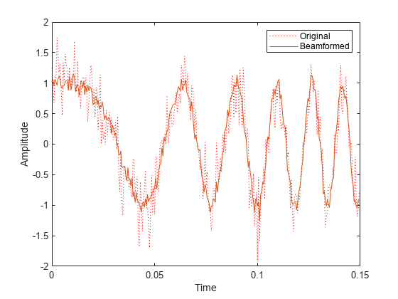
Plot the signal that is input to the middle sensor (channel 6) vs the beamformer output.

plot(t(1:300),real(rx(1:300,6)),'r:',t(1:300),real(y(1:300)))
xlabel('Time')
ylabel('Amplitude')
legend('Original','Beamformed');
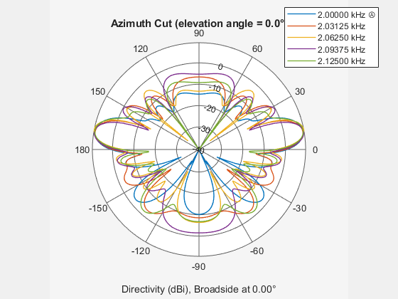
Plot array response

Plot the response pattern for five bands

pattern(array,subbandfreq(1:5).',-180:180,0,...
    'PropagationSpeed',c,'Weights',w(:,1:5));

Apply subband MVDR beamforming to an underwater acoustic 11-element ULA. Beamform the arriving signals to optimize the gain of a linear FM chirp signal arriving from 0 degrees azimuth and 0 degrees elevation. The signal has a bandwidth of 2.0 kHz. In addition, there unit amplitude 2.250 kHz interfering sine wave arriving from 28 degrees azimuth and 0 degrees elevation. Show how the MVDR beamformer nulls the interfering signal. Display the array pattern for several frequencies in the neighborhood of 2.250 kHz. The speed of sound is 1500 meters/sec.

Simulate Arriving Signal and Noise

array = phased.ULA('NumElements',11,'ElementSpacing',0.3);
fs = 2000;
carrierFreq = 2000;
t = (0:1/fs:2)';
sig = chirp(t,0,2,fs/2);
c = 1500;
collector = phased.WidebandCollector('Sensor',array,'PropagationSpeed',c,...
    'SampleRate',fs,'ModulatedInput',true,...
    'CarrierFrequency',carrierFreq);
incidentAngle = [0;0];
sig1 = collector(sig,incidentAngle);
noise = 0.3*(randn(size(sig1)) + 1j*randn(size(sig1)));

Simulate Interfering Signal

Combine both the desired and interfering signals.

fint = 250;
sigint = sin(2*pi*fint*t);
interfangle = [28;0];
sigint1 = collector(sigint,interfangle);
rx = sig1 + sigint1 + noise;

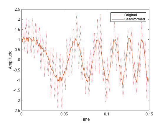
Apply MVDR Beamforming

Use the combined noise and interfering signal as training data.

beamformer = phased.SubbandMVDRBeamformer('SensorArray',array,...
    'Direction',incidentAngle,'OperatingFrequency',carrierFreq,...
    'PropagationSpeed',c,'SampleRate',fs,'TrainingInputPort',true,...
    'NumSubbands',64,...
    'SubbandsOutputPort',true,'WeightsOutputPort',true);
[y,w,subbandfreq] = beamformer(rx,sigint1 + noise);
tidx = [1:300];
plot(t(tidx),real(rx(tidx,6)),'r:',t(tidx),real(y(tidx)))
xlabel('Time')
ylabel('Amplitude')
legend('Original','Beamformed')

Plot Array Response Showing Beampattern Null

Plot the response pattern for five bands near 2.250 kHz.

fdx = [5,7,9,11,13];
pattern(array,subbandfreq(fdx).',-50:50,0,...
    'PropagationSpeed',c,'Weights',w(:,fdx),...
    'CoordinateSystem','rectangular');

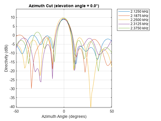
The beamformer places a null at 28 degrees for the subband containing 2.250 kHz.

More About

expand all

Algorithms

expand all

References

[1] Van Trees, H. Optimum Array Processing. New York: Wiley-Interscience, 2002.

Extended Capabilities

Version History

Introduced in R2015b