Main Content

ackermannKinematics

Car-like steering vehicle model

Description

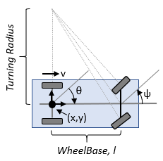
ackermannKinematics creates a car-like vehicle model that uses Ackermann steering. This model represents a vehicle with two axles separated by the distance, WheelBase. The state of the vehicle is defined as a four-element vector, [x y theta psi], with a global xy-position, specified in meters. The xy-position is located at the middle of the rear axle. The vehicle heading, theta, and steering angle, psi are specified in radians. The vehicle heading is defined at the center of the rear axle. Angles are given in radians. To compute the time derivative states for the model, use the derivative function with input steering commands and the current robot state.
Creation

Description

kinematicModel = ackermannKinematics creates an Ackermann kinematic model object with default property values.

example

kinematicModel = ackermannKinematics(Name,Value) sets additional properties to the specified values. You can specify multiple properties in any order.

Properties

expand all

The wheel base refers to the distance between the front and rear axles, specified in meters.

The vehicle speed range is a two-element vector that provides the minimum and maximum vehicle speeds, [MinSpeed MaxSpeed], specified in meters per second.

Object Functions

derivativeTime derivative of vehicle state

Examples

collapse all

Simulate a mobile robot model that uses Ackermann steering with constraints on its steering angle. During simulation, the model maintains maximum steering angle after it reaches the steering limit. To see the effect of steering saturation, you compare the trajectory of two robots, one with the constraints on the steering angle and the other without any steering constraints.

Define the Model

Define the Ackermann kinematic model. In this car-like model, the front wheels are a given distance apart. To ensure that they turn on concentric circles, the wheels have different steering angles. While turning, the front wheels receive the steering input as rate of change of steering angle.

carLike = ackermannKinematics; 

Set Up Simulation Parameters

Set the mobile robot to follow a constant linear velocity and receive a constant steering rate as input. Simulate the constrained robot for a longer period to demonstrate steering saturation.

velo = 5;    % Constant linear velocity 
psidot = 1;  % Constant left steering rate 

% Define the total time and sample rate 
sampleTime = 0.05;                  % Sample time [s]
timeEnd1 = 1.5;                     % Simulation end time for unconstrained robot 
timeEnd2 = 10;                      % Simulation end time for constrained robot 
tVec1 = 0:sampleTime:timeEnd1;      % Time array for unconstrained robot 
tVec2 = 0:sampleTime:timeEnd2;      % Time array for constrained robot  

initPose = [0;0;0;0];               % Initial pose (x y theta phi) 

Create Options Structure for ODE Solver

In this example, you pass an options structure as argument to the ODE solver. The options structure contains the information about the steering angle limit. To create the options structure, use the Events option of odeset and the created event function, detectSteeringSaturation. detectSteeringSaturation sets the maximum steering angle to 45 degrees.

For a description of how to define detectSteeringSaturation, see Define Event Function at the end of this example.

options = odeset('Events',@detectSteeringSaturation);

Simulate Model Using ODE Solver

Next, you use the derivative function and an ODE solver, ode45, to solve the model and generate the solution.

% Simulate the unconstrained robot 
[t1,pose1] = ode45(@(t,y)derivative(carLike,y,[velo psidot]),tVec1,initPose);

% Simulate the constrained robot 
[t2,pose2,te,ye,ie] = ode45(@(t,y)derivative(carLike,y,[velo psidot]),tVec2,initPose,options);

Detect Steering Saturation

When the model reaches the steering limit, it registers a timestamp of the event. The time it took to reach the limit is stored in te.

if te < timeEnd2
    str1 = "Steering angle limit was reached at ";
    str2 = " seconds";
    comp = str1 + te + str2; 
    disp(comp)
end 
Steering angle limit was reached at 0.785 seconds

Simulate Constrained Robot with New Initial Conditions

Now use the state of the constrained robot before termination of integration as initial condition for the second simulation. Modify the input vector to represent steering saturation, that is, set the steering rate to zero.

saturatedPsiDot = 0;             % Steering rate after saturation 
cmds = [velo saturatedPsiDot];   % Command vector 
tVec3 = te:sampleTime:timeEnd2;  % Time vector 
pose3 = pose2(length(pose2),:); 
[t3,pose3,te3,ye3,ie3] = ode45(@(t,y)derivative(carLike,y,cmds),tVec3,pose3,options);

Plot the Results

Plot the trajectory of the robot using plot and the data stored in pose.

figure(1)
plot(pose1(:,1),pose1(:,2),LineWidth=2)
hold on
plot([pose2(:,1); pose3(:,1)],[pose2(:,2);pose3(:,2)])
title("Trajectory X-Y")
xlabel("X")
ylabel("Y") 
legend("Unconstrained Robot","Constrained Robot",Location="northwest")
axis equal

Figure contains an axes object. The axes object with title Trajectory X-Y, xlabel X, ylabel Y contains 2 objects of type line. These objects represent Unconstrained Robot, Constrained Robot.

The unconstrained robot follows a spiral trajectory with decreasing radius of curvature while the constrained robot follows a circular trajectory with constant radius of curvature after the steering limit is reached.

Define Event Function

Set the event function such that integration terminates when 4th state, theta, is equal to maximum steering angle.

function [state,isterminal,direction] = detectSteeringSaturation(t,y)
  maxSteerAngle = 0.785;               % Maximum steering angle (pi/4 radians)
  state(4) = (y(4) - maxSteerAngle);   % Saturation event occurs when the 4th state, theta, is equal to the max steering angle    
  isterminal(4) = 1;                   % Integration is terminated when event occurs 
  direction(4) = 0;                    % Bidirectional termination 

end

References

[1] Lynch, Kevin M., and Frank C. Park. Modern Robotics: Mechanics, Planning, and Control 1st ed. Cambridge, MA: Cambridge University Press, 2017.

Extended Capabilities

C/C++ Code Generation
Generate C and C++ code using MATLAB® Coder™.

Version History

Introduced in R2019b

expand all

Go to top of page