tdr
Description
Use time-domain reflectometry (TDR) to characterize impedance discontinuities from S-parameter data.
Creation
Description
tdrObj = tdr( creates a TDR object
from a Touchstone file or an sparam)sparameters object specified in
sparam to characterize impedance discontinuities in a
system.
Input Arguments
Properties
Object Functions
createTDRTable | Return TDR results as MATLAB table |
plot | Plot TDR response |
tdr.automaticPortOrdering | Display port ordering of S-parameter data |
tdr.sParamQuality | Return S-parameter quality metrics |
Examples
Create an S-parameter object from a 4-port Touchstone file.
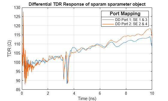
sparam = sparameters('default.s4p');Create a TDR object and set the ConvertToDifferential property to true. In this example, the ports are not defined using the Ports property. Therefore, the tdr object automatically determines the differential ports.
tdrObj = tdr(sparam,'ConvertToDifferential',true);Plot the differential TDR response of a 4-port S-parameter. This plot displays the port mapping between single-ended (SE) ports that the object identified as differential (DD) pairs.
plot(tdrObj)
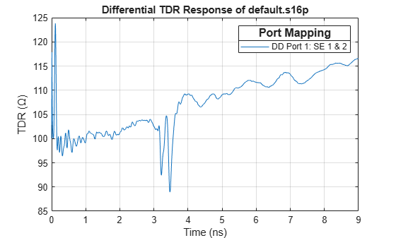
Use a 16-port S-parameter Touchstone file to plot the TDR response of a differential port pair located at port 1 and 2.
First, create a structure to define the rational fitting parameters. These parameters enable you to control the rational fitting process for complex S-parameters.
rationalOptions = struct('Tolerance',-30,'MaxPoles',500);
Create a TDR object with the differential port pair set to 1 and 2.
tdrObj = tdr('default.s16p',...
    ConvertToDifferential=true, ...
    Ports=[1 2],...
    EndTime=9e-9,...
    RiseTime=10e-12,...
    SampleTime=5e-12, ...
    RationalOptions=rationalOptions);
Plot the differential TDR response of the differential port pair 1 and 2.
plot(tdrObj)
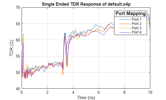
Create a TDR object from a 4-port Touchstone file.
tdrObj = tdr('default.s4p');Plot the single-ended TDR of a 4-port S-parameter in units of impedance.
plot(tdrObj)
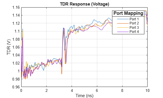
Plot the single-ended TDR of a 4-port S-parameter in units of voltage.
plot(tdrObj, Type="voltage", Title="TDR Response (Voltage)")
Plot the single-ended TDR of a 4-port S-parameter with respect to velocity of propagation of the medium. Scale the X-axis of this response in meters.
plot(tdrObj,Vp=3e8/2,Title="TDR Response(m)")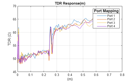
Create a TDR table that displays the time and voltage TDR values for all the ports specified in the TDR object.
T = createTDRTable(tdrObj,tdrType='voltage')T=10000×5 table
Time (s) Port 1 (V) Port 2 (V) Port 3 (V) Port 4 (V)
________ __________ __________ __________ __________
0 1 1 1 1
1e-12 1.0062 0.99943 1.0126 1.0087
2e-12 1.012 0.99992 1.0237 1.0168
3e-12 1.0175 1.0013 1.0335 1.0243
4e-12 1.0228 1.0035 1.0421 1.0312
5e-12 1.0278 1.0063 1.0498 1.0376
6e-12 1.0324 1.0097 1.0565 1.0436
7e-12 1.0369 1.0135 1.0625 1.0491
8e-12 1.041 1.0175 1.0678 1.0541
9e-12 1.0449 1.0218 1.0726 1.0587
1e-11 1.0485 1.0263 1.0769 1.063
1.1e-11 1.0457 1.0313 1.0682 1.0582
1.2e-11 1.043 1.0353 1.0606 1.0536
1.3e-11 1.0404 1.0382 1.0542 1.0494
1.4e-11 1.0378 1.0402 1.0487 1.0453
1.5e-11 1.0353 1.0414 1.044 1.0415
⋮
This example shows computation of time-domain reflectometry (TDR) and group delay of a coaxial transmission line.
Design Coaxial Transmission Line
Design a 75 coaxial transmission line.
Z0 =75; % Desired characteristic impedance (Ohms) innerRadius =
0.0005; % Inner conductor radius (meters) dc = DielectricCatalog; ItemsDC = string(dc.Materials.Name); MaterialType = dielectric(
ItemsDC(5)); % Low loss material
Compute the outer radius of the cable from impedance:
outerRadius = innerRadius*exp(Z0*sqrt(MaterialType.EpsilonR)/60); length =0.01; % Conductor length (meters) mc = MetalCatalog; Items = string(mc.Materials.Name); MetalType = metal(
Items(2));
Create the coaxial transmission line object.
coaxLine = txlineCoaxial( ...
    'InnerRadius', innerRadius, ...
    'OuterRadius', outerRadius, ...
    'LineLength', length, ...
    'EpsilonR', MaterialType.EpsilonR, ...
    'LossTangent', MaterialType.LossTangent,...
    'SigmaCond', MetalType.Conductivity);
Frequency Sweep
Requirements for frequency sweep:
Sweep from DC to very high frequencies to capture details for tdr (frequency to time-domain transformation).
Select a step-size such that the resolution of the frequency sweep ensures the unwrapped phase of S21 decreases with frequency.
travel_time = coaxLine.LineLength*sqrt(coaxLine.EpsilonR)/rf.physconst("LightSpeed");
stepSize = 0.9*(1/(4*travel_time));
freq = stepSize/1e6:stepSize:200e9;
Compute Group Delay
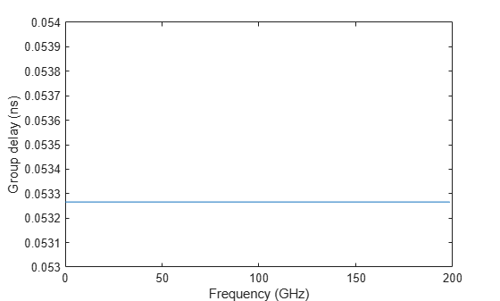
Use the groupdelay function to compute the group delay of the transmission line. Compute the group delay of the transmission line.
gd_ns = groupdelay(coaxLine,freq,"Impedance",Z0)*1e9;Plot the group delay.
plot(freq/1e9, gd_ns)
ylim([floor(min(gd_ns*1e3)) ceil(max(gd_ns*1e3))]./1e3)
ylabel('Group delay (ns)')
xlabel('Frequency (GHz)')
Compute S-parameters
Compute S-parameters of the transmission line for the given frequency sweep and plot S21 phase.
s = sparameters(coaxLine,freq);
rfplot(s,2,1,"angle")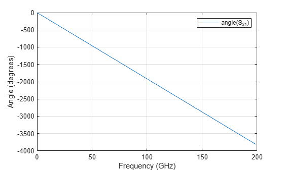
Therefore, we have enough frequency resolution to ensure that the unwrapped phase S21 is decreasing with frequency.
Compute TDR
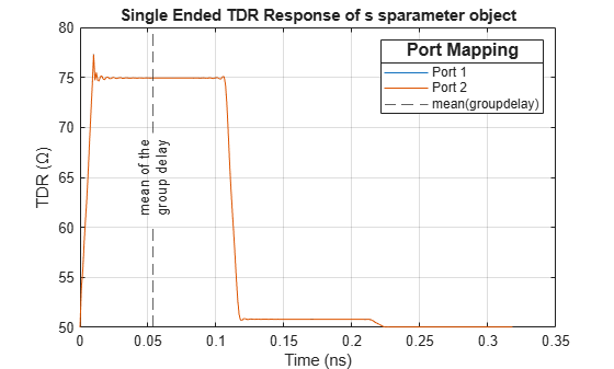
Use tdr function to plot the TDR.
plot(tdr(s,EndTime=(6*travel_time)))
Overlay the mean value of the group delay on the TDR plot.
hold on
xline(mean(gd_ns), '--', {'mean of the','group delay'}, ...
    'DisplayName','mean(groupdelay)',...
    'LabelVerticalAlignment','middle',...
    'LabelHorizontalAlignment','center');
Conclusion
The TDR delay is the time it takes for a signal to enter the input port of the device under test, propagate to the location of a discontinuity, reflect from that discontinuity and then propagate back to the input port. In this case, the discontinuity is the change from the 75 impedance of the DUT to the 50 impedance of the TDR measurement equipment.
Observe that the TDR delay is equivalent to twice the group delay. This observation is generally true for an uniform transmission line, such as a coaxial transmission line, where the:
RLGC is uniformly distributed across the line,
dielectric material is lossless, and
dielectric material has no frequency dependent dispersion.
Therefore, in this study, both TDR delay and group delay represent the time it takes for a signal to traverse the structure, provided the line is uniform and is operating below the multimode threshold.
Version History
Introduced in R2025a