filtfilt
Zero-phase digital filtering
Syntax
Description
y = filtfilt(b,a,x)x in both the forward and reverse directions. After
filtering the data in the forward direction, the function matches initial
conditions to minimize startup and ending transients, reverses the filtered
sequence, and runs the reversed sequence back through the filter. The result has
these characteristics:
Zero phase distortion
A filter transfer function equal to the squared magnitude of the original filter transfer function
A filter order that is double the order of the filter specified by
banda
Do not use filtfilt with differentiator and Hilbert
FIR filters, because the operation of those filters depends heavily on their
phase response.
y = filtfilt(d,x)x using a digital filter
d. Use designfilt to generate
d based on frequency-response specifications.
y = filtfilt(B,A,x,"ctf")x using Cascaded Transfer Functions (CTF) defined by the numerator and denominator coefficients
B and A, respectively. (since R2024b)
Note
Specify the "ctf" option to disambiguate CTF
numerator matrices B with six columns from
second-order section matrix inputs, sos, when you
specify A as a scalar or vector.
y = filtfilt(___,Name=Value)
Examples
Zero-phase filtering helps preserve features in a filtered time waveform exactly where they occur in the unfiltered signal.
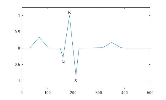
Zero-phase filter a synthetic electrocardiogram (ECG) waveform. The function that generates the waveform is at the end of the example. The QRS complex is an important feature in the ECG. Here it begins around time point 160.
wform = ecg(500);

plot(wform)
axis([0 500 -1.25 1.25])
text(155,-0.4,"Q")
text(180,1.1,"R")
text(205,-1,"S")
Corrupt the ECG with additive noise. Reset the random number generator for reproducible results. Construct a lowpass FIR equiripple filter and filter the noisy waveform using both zero-phase and conventional filtering.
rng("default")

x = wform' + 0.25*randn(500,1);
d = designfilt("lowpassfir", ...
    PassbandFrequency=0.15,StopbandFrequency=0.2, ...
    PassbandRipple=1,StopbandAttenuation=60, ...
    DesignMethod="equiripple");
y = filtfilt(d,x);
y1 = filter(d,x);

tiledlayout("flow")
nexttile
plot([y y1])
title("Filtered Waveforms")
legend(["Zero-phase Filtering" "Conventional Filtering"])

nexttile
plot(wform)
title("Original Waveform")
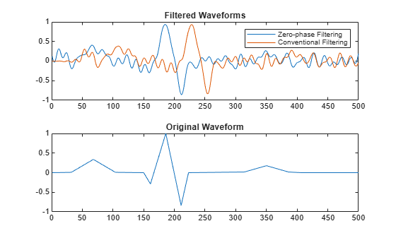
Zero-phase filtering reduces noise in the signal and preserves the QRS complex at the same time it occurs in the original. Conventional filtering reduces noise in the signal, but delays the QRS complex.
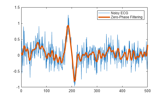
Repeat the filtering using a Butterworth second-order section filter.
d1 = designfilt("lowpassiir",FilterOrder=12, ...
    HalfPowerFrequency=0.15,DesignMethod="butter");
y = filtfilt(d1,x);

figure
plot(x)
hold on
plot(y,LineWidth=3)
hold off
legend(["Noisy ECG" "Zero-Phase Filtering"])
This function generates the ECG waveform.
function x = ecg(L)
%ECG Electrocardiogram (ECG) signal generator.
%   ECG(L) generates a piecewise linear ECG signal of length L.
%
%   EXAMPLE:
%   x = ecg(500).';
%   y = sgolayfilt(x,0,3); % Typical values are: d=0 and F=3,5,9, etc.
%   y5 = sgolayfilt(x,0,5);
%   y15 = sgolayfilt(x,0,15);
%   plot(1:length(x),[x y y5 y15]);

%   Copyright 1988-2002 The MathWorks, Inc.

a0 = [0,1,40,1,0,-34,118,-99,0,2,21,2,0,0,0]; % Template
d0 = [0,27,59,91,131,141,163,185,195,275,307,339,357,390,440];
a = a0/max(a0);
d = round(d0*L/d0(15)); % Scale them to fit in length L
d(15)=L;

for i=1:14
       m = d(i):d(i+1)-1;
       slope = (a(i+1)-a(i))/(d(i+1)-d(i));
       x(m+1) = a(i)+slope*(m-d(i));
end

end
Since R2024b
Use cascaded transfer functions to perform zero-phase filtering.
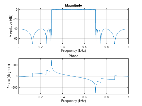
Design an elliptic filter with passband ripple and stopband attenuation of 0.1 dB and 40 dB, respectively. Specify a sample rate of 2000 Hz. Plot the frequency response of the filter.
Fs = 2000;
[B,A] = ellip(20,0.1,40,[0.3 0.7],"ctf");
freqz(B,A,2048,Fs,"ctf")
Filter a linearly swept chirp signal, where the Nyquist frequency occurs at one second. Compare the spectra between the input and output signals.
t = 0:1/Fs:1;
x = chirp(t,0,t(end),Fs/2)';
y = filtfilt(B,A,x,"ctf");
pspectrum([x y],Fs,Leakage=1,FrequencyResolution=1)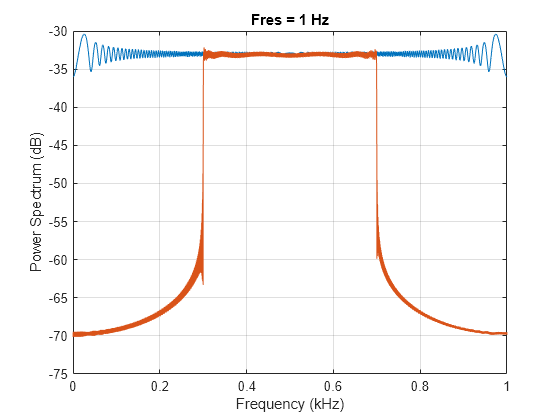
Since R2024b
Recreate noisy sinusoid artifacts with transfer-function zero-phase filtering. Filter an oscillating signal using CTF and scale values.
Create a signal u comprised of normally distributed noise and three sinusoidal waveforms. The sample rate is 1 kHz.
rng("default")
Fs = 1e3;
ts = (0:1/Fs:2)';

a0 = [3 2 1];
f0 = [0.1 0.5 0.9]*Fs/2;
p0 = [0 pi/4 pi/2];

u = 0.1*randn(size(ts)) + 0.1*sin(2*pi*f0.*ts+p0)*a0';
Recreate noisy sinusoid artifacts by filtering n0 with a third-order Butterworth bandstop digital filter and create a signal v.
[b,a] = butter(3,[0.15 0.85],"stop");
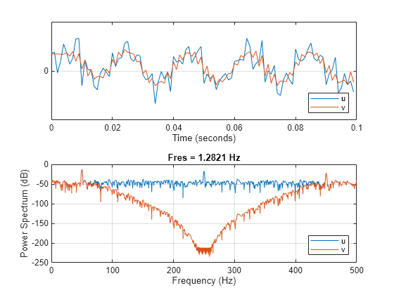
v = filtfilt(b,a,u);Compare u and v. Observe that both signals are in phase.
tiledlayout("flow")
nexttile
strips([u(ts<0.1) v(ts<0.1)],0.1,Fs)
legend(["u" "v"],Location="southeast")
xlabel("Time (seconds)")
nexttile
pspectrum([u v],Fs)
legend(["u" "v"],Location="southeast")
Create a voltage-controlled oscillating signal x. Add noisy sinusoid artifacts represented by the signal v.
vo = exp(-2*abs(ts-1)).*sin(8*pi*ts);
x = vco(vo,[0.25 0.75]*Fs/2,Fs) + v;
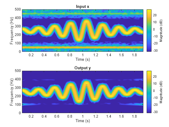
Filter the signal x with a 24th-order Chebyshev type II filter. Use the CTF format and scale values (B,A,g).
[B,A,g] = cheby2(24,50,[0.2 0.8],"ctf");
y = filtfilt({B,A,g},x);
Compare the magnitude squared of the short-time Fourier transforms. Observe a sharp decrease in the magnitude at the stopbands.
tiledlayout("flow")
nexttile
stft(x,Fs,Window=bohmanwin(128),OverlapLength=120, ...
    FFTLength=512,FrequencyRange="onesided")
title("Input x")
nexttile
stft(y,Fs,Window=bohmanwin(128),OverlapLength=120, ...
    FFTLength=512,FrequencyRange="onesided")
title("Output y")
Since R2026a
Apply zero-phase filtering to a complex-valued 30 Hz sinusoidal tone with multiple harmonics at intervals of 60 Hz extending up to 600 Hz.
Create a two-second complex-valued signal with a sample rate of 600 Hz. The signal comprises a 10 V 30 Hz sine tone and has 10 harmonics with frequencies evenly distributed from 60 Hz to 600 Hz with amplitudes of 1 V each.
Fs = 600;
t = (0:1/Fs:2)';
x = 10*exp(1i*2*pi*30*t) + sum(exp(1i*2*pi*60*t*(0:9)),2);
Since the tone oscillates at 30 Hz and the undesired components have frequency peaks at each 60 Hz up to the tenth multiple, a 10th-order IIR comb notch filter is suitable to recover the tone, the signal of interest.
Define b and a as vectors representing the numerator and denominator coefficients of a 10th-order IIR comb notch filter with a quality factor of 35. To learn more about designing IIR comb filters with a specific order and quality factor, see iircomb (DSP System Toolbox).
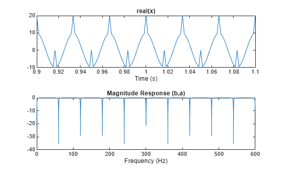
b = [0.957 zeros(1,9) -0.957];
a = [1 zeros(1,9) -0.914];
Plot the real part of the signal from 0.9 to 1.1 seconds. Plot the filter response from 0 to 600 Hz.
tiledlayout("flow")
nexttile
plot(t,real(x))
xlim([0.9 1.1])
xlabel("Time (s)")
title("real(x)")
nexttile
[h,f] = freqz(b,a,8192,"whole",Fs);
plot(f,mag2db(abs(h)))
xlabel("Frequency (Hz)")
title("Magnitude Response (b,a)")
Filter the input signal while preserving the phase. Use Gustafsson's technique to estimate the initial conditions of the filter states. Assume a transient length equal to the signal length and pad the input signal by mirroring its samples.
y = filtfilt(b,a,x, ...
    InitialStatesMethod="gustafsson", ...
    TransientLength=length(x), ...
    PaddingPattern="reflect");
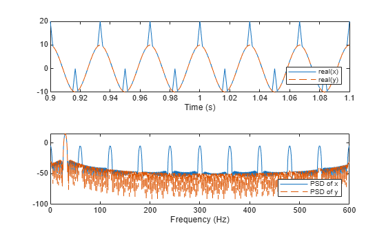
Compare the input and filtered signals in time domain and frequency domain. Plot the real part of both signals from 0.9 to 1.1 seconds, and Welch's power spectra from 0 to 600 Hz. The filtered signal shows the 30 Hz tone with the harmonics removed while the filtered signal y is in phase with the input signal x.
figure;
tiledlayout("vertical")
nexttile
plot(t,real(x),t,real(y),"--")
legend("real(" + ["x" "y"] +")",Location="southeast")
xlabel("Time (s)")
xlim([0.9 1.1])
nexttile
[p,f] = pwelch([x y],[],[],8192,Fs);
pdb = pow2db(abs(p));
plot(f,pdb(:,1),"-",f,pdb(:,2),"--")
xlabel("Frequency (Hz)")
legend("PSD of " + ["x" "y"],Location="southeast")
Input Arguments
Name-Value Arguments
Output Arguments
More About
Tips
You can obtain filters in
CTF format, including the scaling gain. Use the outputs of digital IIR filter design functions,
such as butter, cheby1, cheby2, and ellip. Specify the "ctf" filter-type argument in these
functions and specify to return B, A, and
g to get the scale values. (since R2024b)
References
[1] Gustafsson, F. “Determining the initial states in forward-backward filtering.” IEEE® Transactions on Signal Processing. Vol. 44, April 1996, pp. 988–992. https://doi.org/10.1109/78.492552.
[2] Lyons, Richard G. Understanding Digital Signal Processing. Upper Saddle River, NJ: Prentice Hall, 2004.
[3] Mitra, Sanjit K. Digital Signal Processing. 2nd Ed. New York: McGraw-Hill, 2001.
[4] Oppenheim, Alan V., and Ronald W. Schafer, with John R. Buck. Discrete-Time Signal Processing. 2nd Ed. Upper Saddle River, NJ: Prentice Hall, 1999.