Denoise EEG Signals Using Differentiable Signal Processing Layers

R2026b

This example shows how to remove electro-oculogram (EOG) noise from electroencephalogram (EEG) signals by using the EEGdenoiseNet benchmark data set [1] and deep learning regression. The EEGdenoiseNet data set contains 4514 clean EEG segments and 3400 ocular artifact segments that you can use to synthesize noisy EEG segments with the ground-truth clean EEG.,

In this example, you use clean and EOG-contaminated EEG signals to train a long short-term memory (LSTM) model to remove the EOG artifacts. You first train the model on the raw input signals. Then, you use a short-time Fourier transform (STFT) layer to train the model on the extracted time-frequency features of the input. An inverse STFT layer reconstructs the results from the denoised STFT. Using the time-frequency features improves performance, especially at degraded signal-to-noise ratio (SNR) values.

Create Data Set

The EEGdenoiseNet data set contains 4514 clean EEG segments and 3400 EOG segments that can be used to generate three data sets for training, validating, and testing a deep learning model. The sample rate of all the signal segments is 256 Hz. For convenience, the data set is available at: https://ssd.mathworks.com/supportfiles/SPT/data/EEGEOGDenoisingData.zip

Download the data set by using the downloadSupportFile function.

% Download the data
datasetZipFile = matlab.internal.examples.downloadSupportFile("SPT","data/EEGEOGDenoisingData.zip");
datasetFolder = fullfile(fileparts(datasetZipFile),"EEG_EOG_Denoising_Dataset");
if ~exist(datasetFolder,"dir")     
    unzip(datasetZipFile,fileparts(datasetZipFile));
end

After you download the data, the location in datasetFolder contains two MAT files:

• EEG_all_epochs.mat — A matrix with 4514 clean EEG segments of length 512 samples

• EOG_all_epochs.mat — A matrix with 3400 EOG segments of length 512 samples

Use the createDataset helper function to generate training, validation, and testing data sets. The function combines clean EEG and EOG signals to generate pairs of clean and noisy EEG segments with different SNRs. For any EEG and EOG pair, you can use the following pair of equations to obtain a noisy segment with a given SNR:

$$\text{noisyEEG}=\text{EEG}+\lambda \cdot \text{EOG}$$

$$\text{SNR}=10\cdot {\log }_{10}\left(\frac{\text{rms}\left(\text{EEG}\right)}{\text{rms}\left(\lambda \cdot \text{EOG}\right)}\right)$$

You vary the parameter $\lambda$ to control the artifact power and achieve a particular SNR value.

To create the training data set, createDataset combines the first 2720 pairs of EEG and EOG segments ten times each with random SNRs in the [–7, 2] dB interval for a total of 27,200 training pairs. Each training pair is stored in a MAT file inside a folder named train. Each MAT file includes:

• A clean EEG segment (stored under a variable named EEG)

• An EOG segment (stored under a variable named EOG)

• A noisy EEG segment (stored under a variable named noisyEEG)

• The SNR of the noisy segment (stored under a variable named SNR)

• The sample rate value of the signal segments (stored under a variable named Fs)

To create the validation data set, createDataset combines the next 340 pairs of the EEG and EOG segments ten times each with random SNRs in the [–7, 2] dB interval for a total of 3400 validation segments. Validation data is stored in MAT files inside a folder named validate. Each MAT file contains the same variables as the ones described for the training set.

Finally, to create the test data set, createDataset combines the next 340 pairs of EEG and EOG segments ten times each with deterministic SNR values of –7, –6, –5, –4, –3, –2, –1, 0, 1, and 2 dB. The test data is stored in MAT files inside a folder named test. Test MAT files with the same SNR value are grouped under a common subfolder to make it easier to analyze the denoising performance of the trained model for a given SNR. For example, files with test signals with an SNR of -3 dB are stored in a folder with name data_SNR_-3.

Call the createDataset function to create the data set (this step can take a few seconds). Set the createDatasetFlag to false if you already have the data set in the datasetFolder and want to skip this step.

createDatasetFlag = true;
if createDatasetFlag
    createDataset(datasetFolder);
end

Prepare Datastores to Consume Data

The generated data set is quite large (approximately 430 MB). For convenience, you can use datastores to access the data without reading it all at once into memory. Create signal datastores for the training and validation data. Use the SignalVariableNames parameter to specify the variables you want to read from the MAT files (in the order you want them read). Also specify the ReadOutputOrientation as "row" to ensure the data is compatible with the LSTM network.

ds_Train = signalDatastore(fullfile(datasetFolder,"train"), ...
    SignalVariableNames=["noisyEEG","EEG"], ...
    ReadOutputOrientation="row");
ds_Validate = signalDatastore(fullfile(datasetFolder,"validate"), ...
    SignalVariableNames=["noisyEEG","EEG"], ...
    ReadOutputOrientation="row");

Read the data from the first training file and plot the clean and noisy EEG signals. A call to preview or read methods of the datastore yields a 1-by-2 cell array with the first element containing a noisy EEG segment, and the second element containing a clean EEG segment.

data = preview(ds_Train);
plot([data{2} data{1}],LineWidth=2)
legend("Clean EEG","EEG with EOG artifact")
axis tight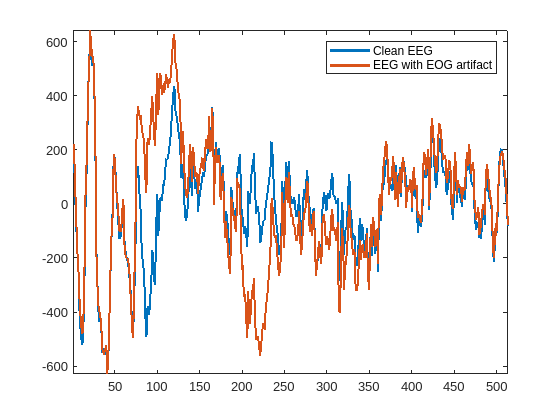

The performance of a regression network usually improves if the input and output signals are normalized. Transform the signal datastores to apply normalization to each signal as it is read from disk. The normalizeData helper function is listed at the end of this example. This function subtracts the signal mean and divides the result by the signal's standard deviation. This is also known as z-score normalization.

ds_Train_T = transform(ds_Train,@normalizeData);
ds_Validate_T = transform(ds_Validate,@normalizeData);

Note that normalization must be applied to input and output signals so it is more convenient to use transformed datastores for this purpose than to use the Normalization="zscore" option of the sequenceInputLayer that only normalizes the inputs.

Train Regression Model to Denoise EEG Signals

Train a model to denoise signals by passing noisy EEG signals into the network input and requesting the desired EEG clean ground-truth signals at the network output. This example uses a long-short term memory (LSTM) architecture because it can learn features from time sequences.

Define the network architecture by setting the number of features to one as a single-channel sequence is input to the network. Use a dropout layer to reduce overfitting of the model on the training data.

numFeatures = 1;
numHiddenUnits = 100;

layers = [
    sequenceInputLayer(numFeatures)
    lstmLayer(numHiddenUnits)
    dropoutLayer(0.2)
    fullyConnectedLayer(numFeatures)
    ];

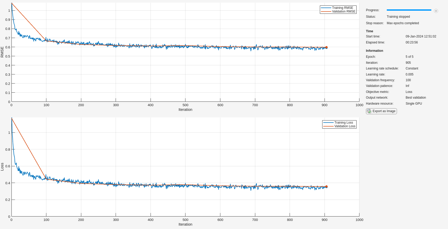
Define the training option parameters. Use an Adam optimizer and shuffle the data every epoch. Display the training progress in a plot and monitor the root mean squared error. Also, specify the validation datastore ds_Validate_T as the source for the validation data.

maxEpochs = 5;
miniBatchSize = 150;

options = trainingOptions("adam", ...
    Metrics="rmse", ...
    MaxEpochs=maxEpochs, ...
    MiniBatchSize=miniBatchSize, ...
    InitialLearnRate=0.005, ...
    GradientThreshold=1, ...
    Plots="training-progress", ...
    Shuffle="every-epoch", ...
    Verbose=false, ...
    ValidationData=ds_Validate_T, ...
    ValidationFrequency=100, ...
    OutputNetwork="best-validation-loss");

Use the trainnet function to train the model. Specify "mse" as the loss function. You can directly pass the transformed training datastore into the function because the datastore outputs a 1-by-2 cell array, with input and output signals, at each call to the read method.

The training steps takes several minutes. You can skip these steps by downloading the two pretrained networks, rawNet and stftNet, using the selector below. If you want to train the network as the example runs, select Train networks. If you want to skip the training steps and download a MAT file containing the pretrained networks, select Download Networks.

trainingFlag = "Train networks";
if trainingFlag == "Train networks"
    rawNet = trainnet(ds_Train_T,layers,"mse",options);
else
    % Download the pretrained networks
    modelsZipFile = matlab.internal.examples.downloadSupportFile("SPT","data/EEGEOGDenoisingNetworks.zip");
    modelsFolder = fullfile(fileparts(modelsZipFile),"EEG_EOG_Denoising_Networks");
    if ~exist(modelsFolder,"dir")
        unzip(modelsZipFile,fileparts(modelsZipFile));
    end
    modelsFile = fullfile(modelsFolder,"trainedNetworks.mat");    
    load(modelsFile)
end

Analyze Denoising Performance of Trained Model

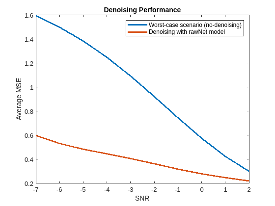
Use the test data set to analyze the denoising performance of the rawNet network. Recall that the test data set contains multiple test files for each SNR value in [–7, –6, –5, –4, –3, –2, –1, 0, 1, 2] dB. For this example, the performance metric is the mean-squared error (MSE) between the clean baseline EEG signal and the denoised EEG signal. Compute the MSE of the clean EEG signal and the noisy EEG signal to show the worst-case MSE when no denoising is applied. At each SNR, compute 340 MSE values for each of the 340 available test EEG segments and obtain the average MSE.

Create a signalDatastore to consume the test data and use a transformed datastore to set up data normalization. Since the data is now inside subfolders of the test folder, specify IncludeSubfolders as true. Then use the folders2labels function to get the list of folder names for each file in the test data set so that you can get data for each SNR.

ds_Test = signalDatastore(fullfile(datasetFolder,"test"), ...
    SignalVariableNames=["noisyEEG","EEG"], ...
    IncludeSubfolders=true, ...
    ReadOutputOrientation="row");
ds_Test_T = transform(ds_Test,@normalizeData);

% Get labels that contain the SNR value for each file in the datastore
labels = folders2labels(ds_Test);
unique(labels)

ans = 10×1 categorical array
    "data_SNR_-1"
    "data_SNR_-2"
    "data_SNR_-3"
    "data_SNR_-4"
    "data_SNR_-5"
    "data_SNR_-6"
    "data_SNR_-7"
    "data_SNR_0"
    "data_SNR_1"
    "data_SNR_2"

For each SNR value, denoise the test signals and compute the average MSE value. Use the subset function of the datastore to get a datastore pointing to the data for each SNR. To denoise a signal, call the minibatchpredict function. Pass the trained network and the noisy data as inputs to minibatchpredict.

SNRs = (-7:2);
MSE_Denoised_rawNet = zeros(numel(SNRs),1); % Measure denoising performance
MSE_No_Denoise = zeros(numel(SNRs),1); % Measure worst-case MSE when no denoising is applied

for idx = 1:numel(SNRs)
    lblIdx = find(labels == "data_SNR_"+num2str(SNRs(idx)));
    ds_Test_SNR = subset(ds_Test_T,lblIdx); % New datastore pointing to files with current SNR value

    % Denoise the data using the minibatchpredict function of the trained model
    pred = minibatchpredict(rawNet,ds_Test_SNR,UniformOutput=false);

    % Use a signal datastore to loop over the 340 denoised signals for the
    % current SNR value. Transform the datastore to add the normalization
    % step. 
    ds_Pred = transform(signalDatastore(pred),@normalizeData);   

    mse = 0;
    mseWorstCase = 0;
    cnt = 0;
    while hasdata(ds_Pred)

        testData = read(ds_Test_SNR);
        denoisedData = read(ds_Pred);

        % MSE performance of denoiser - testData{2} contains clean EEG,
        % testData{1} contains noisy EEG.
        mse = mse + sum((testData{2} - denoisedData).^2)/numel(denoisedData);

        % Worst-case MSE performance when no denoising is applied. 
        % Convert data to single precision as denoisedData is single
        % precision.
        mseWorstCase = mseWorstCase + sum((single(testData{2}) - single(testData{1})).^2)/numel(testData{1});
        cnt = cnt+1;
    end

    % Average MSE of denoised signals
    MSE_Denoised_rawNet(idx) = mse/cnt;

    % Worst-case average MSE
    MSE_No_Denoise(idx) = mseWorstCase/cnt;
end

Plot the average MSE results.

figure
plot(SNRs,[MSE_No_Denoise,MSE_Denoised_rawNet],LineWidth=2)
xlabel("SNR")
ylabel("Average MSE")
title("Denoising Performance")
legend("Worst-case scenario (no-denoising)","Denoising with rawNet model")

Improve Performance Using Feature Extraction

A common approach to improve performance of a deep learning model is to train the network using features of the input signal data. The features provide a representation of the input data that makes it easier for the network to learn the most important aspects of the signals.

Choose a short-time Fourier transformation (STFT) with a window length of 64 samples and overlap length of 63 samples. This transformation effectively creates 33 complex features with a length of 449 samples each.

winLength = 64;
overlapLength = 63;

Compute and plot the STFT of a pair of clean and noisy EEG signals that have been normalized.

data = preview(ds_Train_T);
plotSTFT(data,winLength,overlapLength)

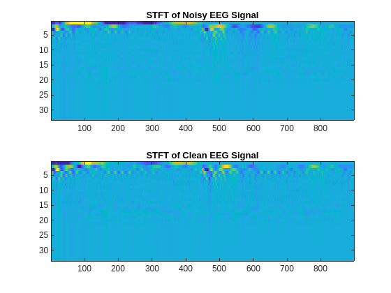
The idea is to train a network so that it can produce a denoised signal based on the STFT of the noisy input signal.

Modify the existing network. Insert an STFT layer so that the network obtains the STFT of the input data. Set the layer transform mode to "realimag". The layer concatenates the real and imaginary parts of the STFT in the channel dimension of the layer output. To reconstruct the signal from the denoised STFT obtained by the network, insert an ISTFT layer after the fully connected layer. Set the output size of the fully connected layer to 66, so that the output size of the ISTFT layer matches the input size to the STFT layer.

minLen=512;                % signal length
numFeatures=66;            % number of features
win=rectwin(winLength);    % analysis window

layers = [
    sequenceInputLayer(1,MinLength=minLen)
    stftLayer(Window=win,OverlapLength=overlapLength,transform="realimag")
    lstmLayer(numHiddenUnits)
    dropoutLayer(0.2)
    fullyConnectedLayer(numFeatures)
    istftLayer(Window=win,OverlapLength=overlapLength)
    ];

Train the network if trainingFlag is "Train networks".

if trainingFlag == "Train networks"
    stftNet = trainnet(ds_Train_T,layers,"mse",options);
end

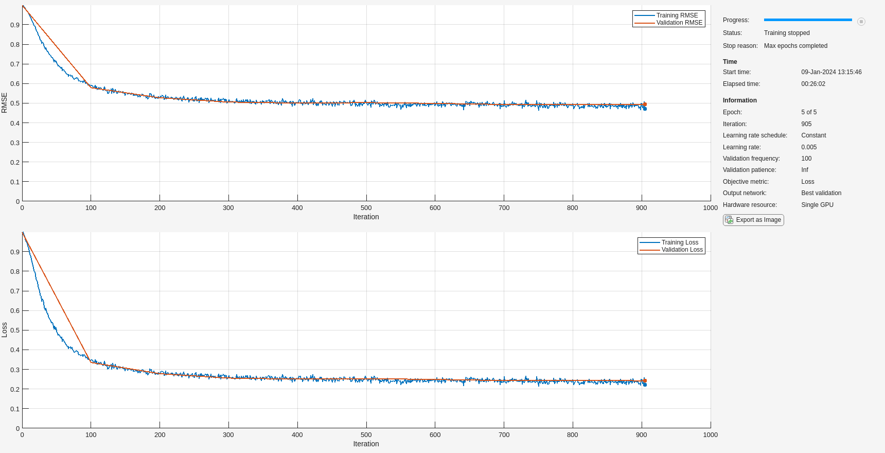
Apply the trained network to denoise EEG signals in the test data. Compute average MSE values by comparing denoised and clean baseline EEG signals.

MSE_Denoised_stftNet = zeros(numel(SNRs),1); % Measure denoising performance
for idx = 1:numel(SNRs)
    lblIdx = find(labels == "data_SNR_"+num2str(SNRs(idx)));
    % New datastores pointing to files with current SNR value
    ds_Test_SNR = subset(ds_Test_T,lblIdx); % Raw EEG signals to compute MSE
    
    % Denoise the data using the predict function of the trained model. 
    pred = minibatchpredict(stftNet,ds_Test_SNR,UniformOutput=false);

    % Use a signal datastore to loop over the 340 denoised signals for the
    % current SNR value.
    ds_Pred = signalDatastore(pred);   

    mse = 0;   
    cnt = 0;
    while hasdata(ds_Pred)

        testData = read(ds_Test_SNR);
        denoisedData = read(ds_Pred);

        % MSE performance of denoiser - testData{2} contains clean EEG
        mse = mse + sum((testData{2}(:) - denoisedData(:)).^2)/numel(denoisedData);
        cnt = cnt+1;
    end

    % Average MSE of denoised signals
    MSE_Denoised_stftNet(idx) = mse/cnt;
end

Compare Results

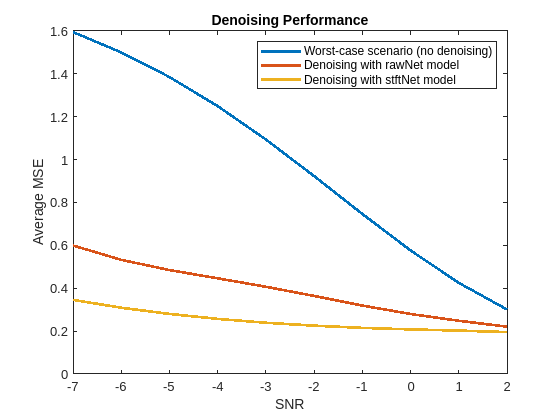
Plot the average MSE obtained with no denoising, denoising with a network trained with raw input signals, and denoising with a network trained with STFT transformed signals. You can see that the addition of the STFT step has improved the performance, especially at the lower SNR values.

figure
plot(SNRs, ...
    [MSE_No_Denoise,MSE_Denoised_rawNet,MSE_Denoised_stftNet], ...
    LineWidth=2)
xlabel("SNR")
ylabel("Average MSE")
title("Denoising Performance")
legend("Worst-case scenario (no denoising)", ...
    "Denoising with rawNet model", ...
    "Denoising with stftNet model")

Plot noisy and denoised signals for different SNRs. The getRandomEEG helper function listed at the end of this example gets a random EEG signal with a specified SNR from the test data.

SNR = -7; % dB
data = getRandomEEG(datasetFolder,SNR);
noisyEEG = normalizeData(data{1});
cleanEEG = normalizeData(data{2});
denoisedEEG = minibatchpredict(stftNet,noisyEEG);

plot([cleanEEG denoisedEEG noisyEEG],LineWidth=2)
title("EEG denoising (SNR = " + SNR + " dB)")
legend("Clean EEG", "Denoised EEG","Noisy EEG")
axis tight

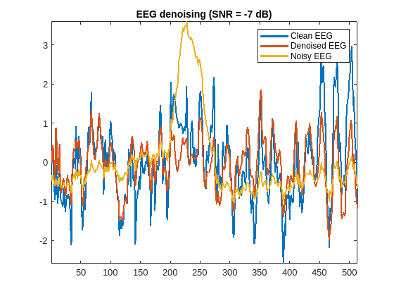
The use of STFT sequences provides greater performance improvement at worse SNRs and both approaches converge in performance as the SNR improves.

References

[1] Haoming Zhang, Mingqi Zhao, Chen Wei, Dante Mantini, Zherui Li, Quanying Liu. "A benchmark dataset for deep learning solutions of EEG denoising." https://arxiv.org/abs/2009.11662

Helper Functions

normalizeData - this function normalizes input signals by subtracting the mean and dividing by the standard deviation.

function y = normalizeData(x)
% This function is intended only to support examples in Signal
% Processing Toolbox. It may be changed or removed in a future release.

if iscell(x)
    y = cell(1,numel(x));
    y{1} = (x{1}-mean(x{1}))/std(x{1});

    if numel(x) == 2
        y{2} = (x{2}-mean(x{2}))/std(x{2});
    end
else
    y = (x - mean(x))/std(x);
end
end

plotSTFT - this function plots the short-time Fourier transform (STFT) of the input data. It converts the complex STFT results into a real matrix by concatenating the real and imaginary components.

function plotSTFT(data,winLength,overlapLength)
% This function is intended only to support examples in Signal
% Processing Toolbox. It may be changed or removed in a future release.
dataNoisy = data{1};
dataClean = data{2};
y = stft([dataNoisy dataClean],Window=rectwin(winLength), ...
    OverlapLength=overlapLength, ...
    FrequencyRange="onesided");
stftNoisy = y(:,:,1);
stftClean = y(:,:,2);
tiledlayout(2,1)
nexttile
h = imagesc([real(stftNoisy) imag(stftNoisy)]);
h.Parent.CLim = [-40 57];
title("STFT of Noisy EEG Signal")
nexttile
h = imagesc([real(stftClean) imag(stftClean)]);
h.Parent.CLim = [-40 57];
title("STFT of Clean EEG Signal")
end

createDataset - this function combines clean EEG signal segments with EOG segments to create training, validation and testing datasets to train an EEG denoiser neural network.

function createDataset(dataDir)
% This function is intended only to support examples in Signal
% Processing Toolbox. It may be changed or removed in a future release.

% Create training, validation, and testing datasets consisting of clean EEG
% signals and noisy EEG signals contaminated by EOG segments. 

load(fullfile(dataDir,"EEG_all_epochs.mat"),"EEG_all_epochs");
load(fullfile(dataDir,"EOG_all_epochs.mat"),"EOG_all_epochs");

EEG_all_epochs = EEG_all_epochs(1:3400,:).';
EOG_all_epochs = EOG_all_epochs.';
Fs = 256;
trainingPercentage = 80;
validationPercentage = 10;
N = size(EEG_all_epochs,2);

% Create a training data set consisting of MAT files containing two
% signals: a clean EEG signal, and an EEG signal contaminated by EOG artifacts.
% Combine each of 2720 pairs of EEG and EOG segments ten times with random
% SNRs in the -7dB to 2dB range to obtain 27200 training segments.

EEG_training = EEG_all_epochs(:,1:N*trainingPercentage/100);
EOG_training = EOG_all_epochs(:,1:N*trainingPercentage/100);

M = size(EEG_training,2);
cnt = 0;
if ~exist(fullfile(dataDir,"train"),'dir')
    mkdir(fullfile(dataDir,"train"))
end
for idx = 1:M
    for kk = 1:10
        cnt = cnt + 1;
        EEG = EEG_training(:,idx);
        EOG = EOG_training(:,idx);
        [noisyEEG,SNR] = createNoisySegment(EEG,EOG,[-7,2]);
        save(fullfile(dataDir,"train", ...
            "data_" + num2str(cnt) + ".mat"), ...
            "EEG","EOG","noisyEEG","Fs","SNR");
    end
end

% Create a validation data set by combining 340 pairs of EEG and EOG
% segments ten times with random SNRs in (-7:2) dB
tPer = trainingPercentage/100;
vPer = validationPercentage/100;

EEG_validation = EEG_all_epochs(:,1+N*tPer:N*tPer+N*vPer);
EOG_validation = EOG_all_epochs(:,1+N*tPer:N*tPer+N*vPer);

M = size(EEG_validation,2);
cnt = 0;
if ~exist(fullfile(dataDir,"validate"),'dir')
    mkdir(fullfile(dataDir,"validate"))
end
for idx = 1:M
    for kk = 1:10
        cnt = cnt + 1;
        EEG = EEG_validation(:,idx);
        EOG = EOG_validation(:,idx);
        [noisyEEG,SNR] = createNoisySegment(EEG,EOG,[-7,2]);
        save(fullfile(dataDir,"validate", ...
            "data_" + num2str(cnt) + ".mat"), ...
            "EEG","EOG","noisyEEG","Fs","SNR");
    end
end

% Create a test data set by combining 340 pairs of EEG and EOG segments ten
% times with 10 SNR values [-7 -6 -5 -4 -3 -2 -1 0 1 2] dB. Store the
% training sets in folders with names that identify the SNR value so that
% it is easy to analyze performance by accessing files with a specific SNR.

EEG_test = EEG_all_epochs(:,1+N*tPer+N*vPer:end);
EOG_test = EOG_all_epochs(:,1+N*tPer+N*vPer:end);

M = size(EEG_test,2);
SNRVect = (-7:2);
for kk = 1:numel(SNRVect)
    cnt = 0;
    if ~exist(fullfile(dataDir,"test","data_SNR_" + num2str(SNRVect(kk))),'dir')
        mkdir(fullfile(dataDir,"test","data_SNR_" + num2str(SNRVect(kk))));
    end
    for idx = 1:M
        cnt = cnt + 1;
        EEG = EEG_test(:,idx);
        EOG = EOG_test(:,idx);
        [noisyEEG,SNR] = createNoisySegment(EEG,EOG,SNRVect(kk));
        save(fullfile(dataDir,"test", ...
            "data_SNR_" + num2str(SNR)+"/" + "data_"+num2str(cnt) + ".mat"), ...
            "EEG","EOG","noisyEEG","Fs","SNR");
    end
end
end

function [y,SNROut] = createNoisySegment(eeg,artifact,SNR)
% Combine EEG and artifact signals with a specified SNR in dB. If SNR is a
% two-element vector, its value is chosen randomly from a uniform
% distribution over the interval [SNR(1) SNR(2)].

if numel(SNR) == 2
    SNR = SNR(1) + (SNR(2)-SNR(1)).*rand(1,1);
end

k = 10^(SNR/10);
lambda = (1/k)*rms(eeg)/rms(artifact);

y = eeg + lambda * artifact;

SNROut = SNR;
end

The getRandomEEG function reads the data from a random EEG test file with a specified SNR.

function data = getRandomEEG(datasetFolder,SNR)
sds  = signalDatastore(fullfile(datasetFolder,"test","data_SNR_"+num2str(SNR)), ...
    SignalVariableNames=["noisyEEG","EEG"],IncludeSubfolders=true);
n = numel(sds.Files);
idx = randi(n,1);
data = read(subset(sds,idx));
end