Using Network Couplers to Split Physical Networks
Why Use Network Couplers?
When modeling a complete physical system, the models can become quite large, resulting in longer simulation times. This can become problematic when you need to deploy the physical model to real time for hardware-in-the-loop studies. It can also be an issue for desktop simulation when you need to explore multiple scenarios or design options.
In such cases, the best first step is always to reduce modeling fidelity to the minimum level needed. For example, if modeling an electric vehicle drive cycle, there is no need to model the switching of power electronics because average value or energy-balancing methods should be sufficient. Use the detailed switching power electronics models in separate test harnesses to determine average losses to be used at the system level.
For some systems, however, this is not enough. Even when modeled at a requisite level of detail, system complexity is sometimes too high to run the complete model on a single microprocessor in real time. In this case, you need to split the model into smaller pieces that can be deployed to multiple processors. The blocks in the Network Couplers library help you do that.
A Simscape™ network cannot be directly divided into separate parts for simulation on different processors. This is because the network is parsed, simplified, and presented to the solver as a single entity. Therefore, you need to split your Simscape network into separate smaller networks interfaced to each other through Simulink® connections. The Simscape Network Couplers library provides the starting point for you to do this. The blocks in the library look like standard Simscape blocks (for example, Inductor), but are actually subsystems that implement the network separation. The design of the coupler blocks enables you to iterate on where to divide your model without initially changing its architecture.
Naming Conventions
Once you use the network coupler blocks to split a Simscape network in your model into multiple coupled networks, each of these networks can have its own solver settings. For example, you can use a variable solver for one of the coupled networks and a fixed-step solver for another, or use two fixed-step solvers with different step sizes. This makes it easier to deploy your system for hardware-in-the-loop simulation.
For clarity, the block interface and the documentation use these naming conventions for coupled networks:
| Network Coupling Scenario | Naming Convention |
|---|---|
One network is variable-step and the other is fixed-step |
|
Both networks are fixed-step, with different step sizes |
|
When using the network coupler blocks, connect port 1 of the block to Network 1 and port 2 to Network 2.
If both networks are variable-step, or both networks are fixed-step with the same step size, then the block orientation does not matter.
Best Practices for Splitting Physical Networks
Deciding where to split a network requires some thought. Ultimately, you are looking to balance the computational burden evenly across two or more microprocessors. However, to minimize loss of modeling fidelity and to reduce likelihood of numerical instability, you also want to split the network at places where there are no fast dynamics.
When interfacing the separated networks, it is necessary to introduce some dynamics or delays to remove any algebraic constraints, which may lead to the loss of fidelity or instability issues. One approach to mitigate these issues is to select a dynamic component in the system as a splitting point and use its time constant to remove the algebraic loop. Suitable components include inductors, flexible shafts, and compressible volumes of fluid.
Also, avoid splitting the network at a point where there is high-frequency activity. For example, in a power network, split at a DC link rather than an AC link if you have the choice.
About the Network Couplers Library
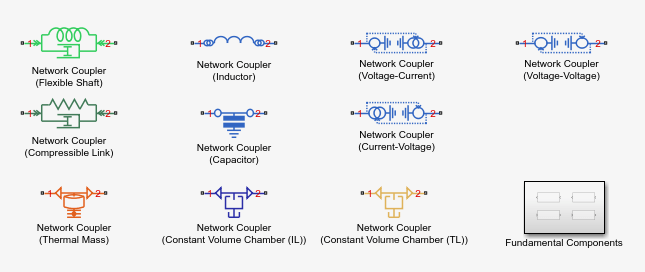
The Network Couplers library, available as a sublibrary in the Utilities library, contains network coupler blocks for mechanical, electrical, thermal, and fluid domains:
| Domain | Network Coupler Blocks |
|---|---|
Mechanical Rotational | Network Coupler (Flexible Shaft) |
Mechanical Translational | Network Coupler (Compressible Link) |
Electrical | Network Coupler (Inductor) Network Coupler (Capacitor) Network Coupler (Voltage-Current) Network Coupler (Current-Voltage) Network Coupler (Voltage-Voltage) |
Thermal | Network Coupler (Thermal Mass) |
Isothermal Liquid | Network Coupler (Constant Volume Chamber (IL)) |
Thermal Liquid | Network Coupler (Constant Volume Chamber (TL)) |
For the electrical domain, the library provides several blocks for use in a variety of scenarios:
| Block Name | When To Use | Limitations |
|---|---|---|
Network Coupler (Inductor) | Circuit has an inductor at the point where you want to split the network. |
|
Network Coupler (Capacitor) | Circuit has a capacitor (connected to an electrical reference) at the point where you want to split the network. This block can be useful for connecting ground planes or return paths. | Make sure that the RC time constant, which results from the capacitor and the connected network series resistances, is not faster than can be tracked by the simulation step size. |
Network Coupler (Voltage-Current) | Network 1 has series-connected inductors or current sources, while Network 2 models something like a capacitive load or battery. | Changes the behavior of the system because it adds a first-order lag to break the algebraic loop. |
Network Coupler (Current-Voltage) | Network 2 has series-connected inductors or current sources, while Network 1 models something like a capacitive load or battery. | Changes the behavior of the system because it adds a first-order lag to break the algebraic loop. |
Network Coupler (Voltage-Voltage) | Both networks have series-connected inductors or current sources. | Some experimentation may be required to find good values for the internal source resistances. Accuracy is not as good as when splitting the network using an inductor or capacitor. |
The block icons are similar to the equivalent Foundation library blocks, but have small annotations to indicate whether they act internally as Through or Across sources. These annotations help when deciding which coupler block to use. For example, the Network Coupler (Inductor) block icon shows the standard inductor symbol with two overlapping circles adjacent to each port, to indicate two internal current sources. Therefore, you should never connect the Network Coupler (Inductor) block directly to a current source, or to another inductor. For more information, see Avoiding Numerical Simulation Issues.
Additionally, the Network Couplers library contains a Fundamental Components sublibrary with prediction and smoothing blocks. For more information, see Prediction and Smoothing.
General Principles of Using the Network Couplers Blocks
The blocks in the Network Couplers library look like standard Simscape blocks, but are actually subsystems that implement the network separation.
When you add a Network Couplers library block to your model, the library links are broken. This means that you can customize the coupler blocks and associated subsystem contents, if needed.
When you double-click a coupler block in your model, the underlying subsystem opens. It generally contains two masked subsystems, Port 1 Interface and Port 2 Interface, connected to each other through two rate transition blocks. By default, the rate transition blocks are commented through. Uncomment them if at least one of the coupled networks is running fixed step.
Masking the Port 1 Interface and Port 2 Interface subsystems, rather than the top-level network coupler subsystem, helps with restructuring the model into different task subsystems for real-time deployment.
Sampling Types
All of the coupler blocks have some common options and parameters to specify the sampling types of the two connected networks. The table shows the possible scenarios.
| Case | Network 1 | Network 2 |
|---|---|---|
1 | Variable-step | Variable-step |
2 | Variable-step | Fixed-step |
3 | Fixed-step, step size h | Fixed-step, step size h |
4 | Fixed-step, step size h1 | Fixed-step, step size h2, where h2>h1 |
In cases 1 and 3 both networks have the same sampling type. However, for cases 2 and 4, the sampling types differ, and Network 1 is the faster network (as described in Naming Conventions), that is, its solver takes smaller steps. The Port 1 Interface block implements the dynamic breaking of the Simulink algebraic loop because the smaller time step supports a faster time constant and less loss of accuracy.
In the Port 1 Interface block dialog, set the Sampling type parameter to match your network sampling scenario:
Variable step at ports 1 and 2— Both networks are variable-step.Variable step at port 1 and fixed step at port 2— Network 1 is variable-step and Network 2 is fixed-step.Fixed step both ports with common sample time— Both networks are fixed-step, with the same step size.Fixed step both ports with faster sampling at port 1— Both networks are fixed-step, with different step sizes.
The parameter list changes, based on the selected option. Set the other parameter values, as needed. Use the Analysis > Derived values section of the block dialog to look up recommended values.
Prediction and Smoothing
Connecting a network with faster sampling (Network 1) to a network with slower sampling (Network 2) may result in accuracy loss in the Network 1 simulation when its sample times are between the sample times of Network 2. The Prediction (slow->fast) block helps prevent the accuracy loss. It predicts the output of Network 2 between its sample times by using the last computed derivative of the output of Network 2. The block implementation is a masked subsystem.
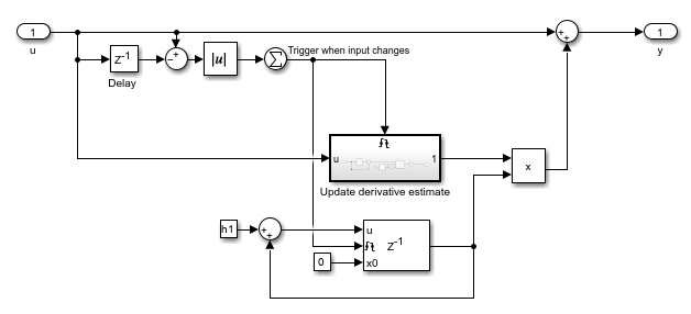
The subsystem contains blocks that run at both the slower and the faster rate. The Delay block is driven by the slower rate, and changes in its output are used as a trigger, so that the triggered subsystem captures the latest derivative of input u. The discrete-time integrator runs at the faster rate and uses this derivative to predict the output y until the next trigger event happens.
The Prediction (discrete->continuous) block works in a similar fashion to provide estimates for the case when Network 1 is variable-step and Network 2 is fixed-step.
When Network 1 has high-frequency activity above what Network 2 can sample, applying smoothing to the output of Network 1 can sometimes be advantageous because it helps you avoid picking a local peak or trough of the Network 1 activity. The Smoothing (fast->slow) block provides an averaged value of the Network 1 output to Network 2. The block implementation is also a masked subsystem.
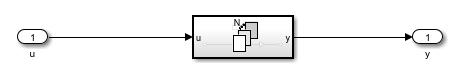
The smoothing works by averaging the last N samples. You specify N by using the Number of samples over which to smooth parameter.
The Smoothing (continuous->discrete) block is intended for when Network 1 is variable-step and Network 2 is fixed-step. Instead of averaging, the block uses a first-order filter to remove unwanted high-frequency information.
These prediction and smoothing algorithms are built into the Network Coupler blocks, and you can enable them by using the check boxes in the block dialogs. The prediction and smoothing blocks in the Fundamental Components sublibrary are provided for your reference.
Typical Workflow
This is the recommended workflow for dividing a network:
Create a baseline simulation and save associated results, to later validate the divided network against these results. Usually this step is done with the Simscape network simulated using a variable-step solver, for best accuracy.
Identify a suitable place to split the network. If possible, select an existing system component for which there is an equivalent in the Network Couplers library. Also try to avoid splitting the network at places where there is high-frequency activity. For more information, see Best Practices for Splitting Physical Networks.
Replace the existing component with the equivalent from the Network Couplers library and set parameters accordingly, or add a new component. Also remember to add a Solver Configuration block to the part of the network that does not have one after splitting.
Pay particular attention to setting of correct initial conditions for the coupler blocks. One way to get initial conditions is to extract them from the baseline in Step 1.
Run the simulation again, still using variable-step solver, and validate the results against the baseline. If you replaced an existing component, results should be the same. If you added a component, the simulation results will differ, in which case use this step to determine acceptable parameter values for the added component.
Change the sampling types for the two connected networks to the values you expect to use. To switch a Simscape network to using a fixed-step solver, open its Solver Configuration block, select the Use local solver check box, and use the Sample time parameter to specify the sample time.
Change the Sampling type parameter value of the coupler block to match the sampling types of the two networks. Uncomment the rate transition blocks in the top-level subsystem of the coupler block.
Run the simulation and compare to the baseline, and make adjustments to the sample times if necessary. Use the Analysis tab of the coupler block to get information about suggested maximum sampling times.
Check to see if prediction or smoothing can help in your application by selecting and clearing the corresponding check boxes in the coupler block dialog.
When satisfied with the simulation results, redraw the block diagram by expanding the Network Coupler subsystems and moving them up one level, to make the Simulink connections visible at the top level of the block diagram, along with the rate transition blocks. You can then group the blocks and subsystems by sampling times and perform other steps needed for deployment to a multirate HIL platform, the same way as for any other Simulink model.
For a detailed example of splitting an electrical vehicle model into separate networks and then deploying it to a multirate HIL, see Configuring an EV Simulation for Multirate HIL.
See Also
Network Coupler (Compressible Link) | Network Coupler (Flexible Shaft) | Network Coupler (Inductor) | Network Coupler (Capacitor) | Network Coupler (Current-Voltage) | Network Coupler (Voltage-Current) | Network Coupler (Voltage-Voltage) | Network Coupler (Thermal Mass) | Network Coupler (Constant Volume Chamber (IL)) | Network Coupler (Constant Volume Chamber (TL))