Model Conveyor Belt as Cyber-Physical System

This example shows how to model a variable-speed conveyor belt as a cyber-physical system by combining continuous-time, discrete-event, and finite-state modeling techniques. The model in this example integrates the modeling techniques required to represent the cyber-physical system into a single simulation environment by using Simulink®, SimEvents®, and Stateflow®.

This example uses blocks from both SimEvents and Stateflow. If you do not have a license for either SimEvents or Stateflow, you can open and simulate the model, but you can only make basic changes to the model, such as modifying block parameters.

Open and Explore Conveyor Belt Model

Cyber-physical systems combine computer systems and physical systems to achieve design goals. The model in this example represents a variable-speed conveyor belt system. The conveyor belt moves human passengers and transitions to three different operational modes based on the load of passengers on the conveyor belt.

• An Entity Generator block creates SimEvents entities to model passengers on the conveyor belt as discrete individuals.

• A Stateflow chart models the transitions between operational modes and the dynamics of the motors that drive the variable-speed conveyor belt.

• An Entity Transport Delay block connects the continuous-time domain to the discrete-event and finite-state domains by modeling the passenger throughput as a function of the runtime conveyor belt dynamics.

Open the model VariableSpeedConveyorBelt.

mdl = "VariableSpeedConveyorBelt";
open_system(mdl)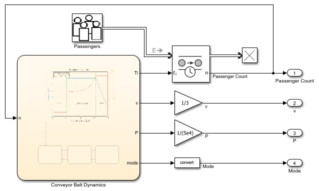

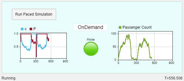
A dashboard for simulating and monitoring the system opens in a separate window.

Model Passenger Arrivals as Discrete Events

Passengers on the conveyor belt are discrete individuals who arrive independently, and passenger traffic varies over time. To model passengers as discrete and independent, the Entity Generator block produces a SimEvents entity for each passenger. The intergeneration time of the Entity Generator block represents the passenger traffic.

The Entity Generator block in this example models passenger arrival and the variation in passenger traffic as a Poisson process represented by this equation

$P\left(\Delta t\right)=\lambda e^{-\lambda \Delta t}$,

where $\lambda$ represents the arrival rate and $\Delta t$ is the intergeneration time.

The Entity Generator block creates time-based entities using a MATLAB action as the time source. MATLAB code defines the intergeneration time for each entity. To model the variation in passenger traffic throughout the day, the MATLAB code varies the arrival rate $\lambda$ according to this equation.

$$\lambda \left(t\right)=\{\begin{array}{ll}2,& ifmod\left(t,300\right)\in \left[0,180\right)\\ 0.5,& ifmod\left(t,300\right)\in \left[180,240\right)\\ 0.1,& ifmod\left(t,300\right)\in \left[240,300\right)\end{array}$$

The arrival rate cycles with a period of 300. The start of the cycle has the highest arrival rate and corresponds to rush hour traffic. As rush hour concludes, the arrival rate drops to represent normal traffic. At the end of the cycle, the arrival rate drops again to represent low traffic.

Model Conveyor Belt Operation as Finite State Machine

The conveyor belt has one of three modes of operation based on the weight of the load.The graph shows the transfer characteristics of the conveyor belt velocity and power in each operational mode against a logarithmic scale of the load weight.

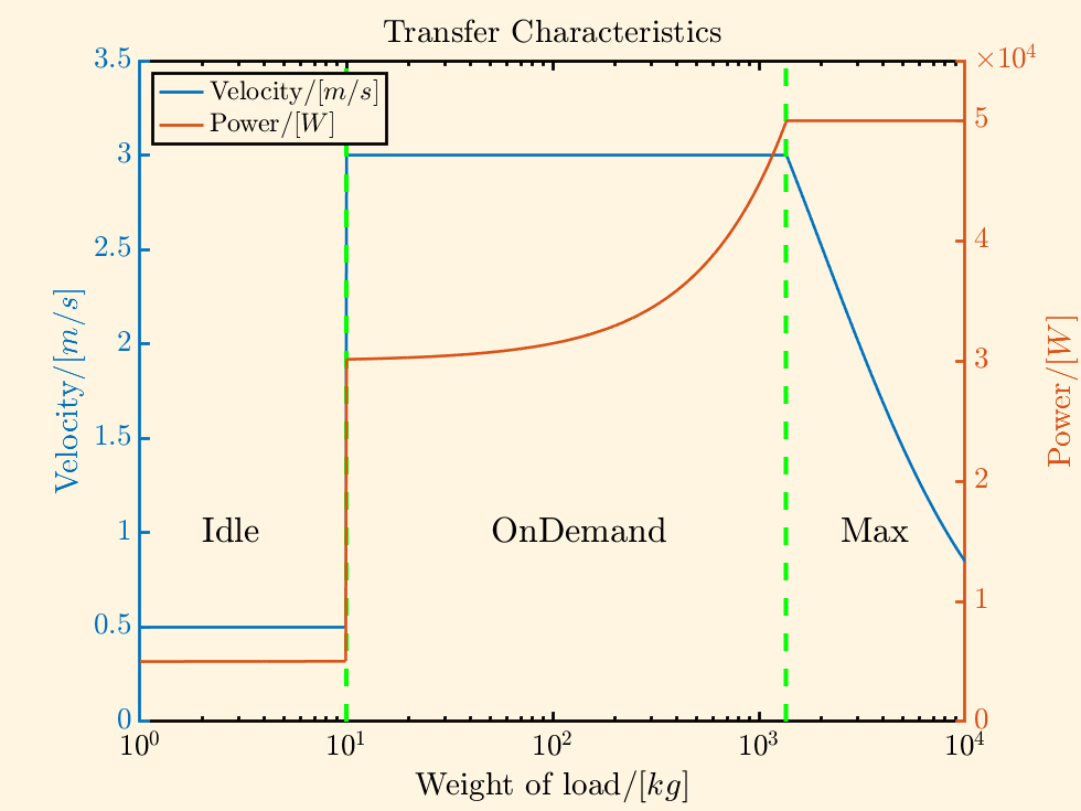
• In the idle operational mode, the weight of the load is low, indicating few or no passengers. The system saves energy by maintaining a low velocity.

• The on demand operational mode represents typical operation. The conveyor belt maintains a velocity of about 3 m/s to optimize passenger comfort and throughput. The power from the motors increases as the weight of the load increases.

• In the max operational mode, the weight of the load is too high for the motors to maintain the optimal velocity. The motors supply constant maximum power output to keep the conveyor belt moving as quickly as possible. As the weight of the load increases, the velocity decreases.

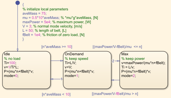
The Stateflow chart computes the motor power and velocity and models the operational modes of the conveyor belt as a finite state machine.

Model Continuous Dynamics of Conveyor Belt

Continuous dynamics govern the way that the conveyor belt moves passengers. For example, the velocity of the conveyor belt determines the time each passenger spends on the conveyor belt. Because the velocity varies dynamically, the transit time for a given passenger can change while the passenger is on the conveyor belt. This variation in transit time means that the continuous dynamics affect the finite-state dynamics in the system. Both the passenger arrival and transit time determine the instantaneous load, which determines the operational mode.

The Entity Transport Delay block models the transit time as a transport delay. In each time step, the Stateflow chart calculates the instantaneous delay $T_i$ for passengers on the conveyor belt based on the current velocity and operational mode. The block uses the instantaneous delays to calculate the transport delay, or total transit time, and determine when each passenger steps off the conveyor belt.

Simulate Conveyor Belt System

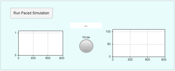
To monitor the system behavior during simulation, use the dashboard to run a paced simulation of the model. In the dashboard, click Run Paced Simulation.

Simulation pacing slows the simulation execution so you can observe the behavior of the system during simulation. This example paces the simulation to an approximate rate of 15 seconds of simulation time per 1 second of wall-clock time so that the 900-second simulation takes about one minute to complete.

As the simulation runs, you can monitor the conveyor belt operation and passenger traffic and throughput in the dashboard.

• A Dashboard Scope block plots the normalized velocity of the conveyor belt and the normalized power output of the conveyor belt motor.

• A Display block and a Lamp block show the operational mode of the conveyor belt.

• Another Dashboard Scope block plots the passenger count over time.

• The status bar below the dashboard shows the simulation status and the simulation time.

Alternatively, to run a simulation without simulation pacing, use one of these options:

• In the Simulink Toolstrip or the toolbar at the top of the dashboard, click Run.

• Run the simulation programmatically using the sim function.

For example, use this command to simulate the model programmatically.

out = sim(mdl);

Analyze Simulation Results

The simulation results are returned as a single Simulink.SimulationOutput object. Get the logged time data and the logged data for the Passenger Count, v, and P outputs.

pcount = getElement(out.yout,"Passenger Count");
v = getElement(out.yout,"v");
P = getElement(out.yout,"P");
t = out.tout;

Plot each signal on its own axes within a vertical tiled layout.

tiledlayout("vertical",TileSpacing="tight",Padding="tight")
nexttile
plot(t,pcount.Values.Data)
ylabel(["Passenger" "Count"])

nexttile
plot(t,v.Values.Data)
ylabel(["Normalized" "Velocity"])
ylim([-0.1 1.1])

nexttile
plot(t,P.Values.Data)
xlabel("Time(s)")
ylabel(["Normalized" "Power"])
ylim([-0.1 1.1])

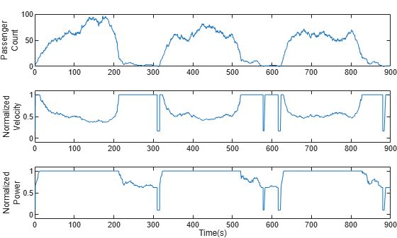
The 900-second simulation covers three cycles of varying passenger traffic. The normalized velocity and power data shows that the conveyor belt moves through three operational cycles that align with the 300-second period of the passenger traffic cycle.

Each cycle starts with rush hour passenger traffic, and the passenger count increases quickly. Initially, the conveyor belt is in the on-demand operational mode. The velocity is constant, and the power output increases with the passenger count.

As passengers continue to arrive, the conveyor belt reaches maximum load and transitions to the max operational mode. The power output remains constant, at the maximum power the motors can provide. The velocity changes as the passenger count and conveyor belt load varies but stays below the optimal velocity of the on-demand operational mode.

Rush hour ends a little over half way through the passenger traffic cycle. As passenger traffic drops, fewer passengers are on the conveyor belt, and the conveyor belt transitions back to the on-demand operational mode. The velocity remains constant, and the power varies with the passenger count.

The end of each cycle has a brief lull in passenger traffic. The conveyor belt briefly transitions to the idle operational mode. The passenger count reaches zero, and the velocity and power both drop to a constant, low value to save energy.