Parameter Estimation with Constraints on Lookup Table Values

The example shows how to perform parameter estimation while also imposing constraints on the parameters being estimated. In this example, you estimate the parameters of a model that contains a nonlinear spring. The parameters in this model are the spring stiffness values, which are contained in a lookup table.

Open Model

The model in this example contains a nonlinear translational spring. Instead of a single spring constant, a lookup table characterizes the nonlinear spring. The table breakpoints consist of the deformation values of the spring, which range from -2 to 2. For each deformation value, there is a spring stiffness value. If the spring had a single spring constant, the stiffnesses would be a linear function of the deformation. However, in this case, the vector of stiffness values does not need to be linear. Nonlinear stiffness values enable you to model, for example, a spring whose stiffness changes as it is stretched or compressed. For more information on the nonlinear translational spring block, see Nonlinear Translational Spring (Simscape Driveline).

To characterize the spring stiffness in the model, you apply a position reference command to a controller that drives the mass to follow the reference command. Open the Simulink® model.

open_system("sdoNonlinearSpringWithController");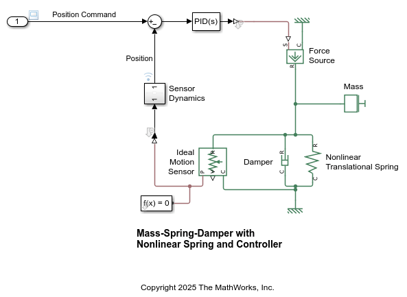

Plot Model Response Before Estimation

Load the input data, output data, and time values.

load("sdoNonlinearSpringWithController_Data.mat","ChirpTime","ChirpInput","ChirpOutput");

To stimulate the model with the input data and compute the model response, use the computeModelResponse helper function, which is provided at the end of the example.

[modelOutputTime,modelOutputData] = computeModelResponse(ChirpTime,ChirpInput,ChirpOutput);

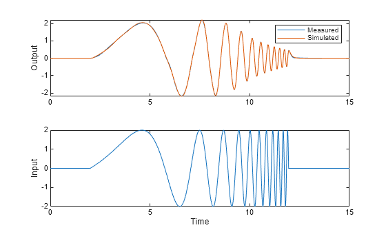
Plot the input and output data. Plot the model response and compare it with the output data.

figure;
subplot(2,1,1);
plot(ChirpTime,ChirpOutput);
hold on;
plot(modelOutputTime,modelOutputData);
legend('Measured','Simulated');
ylabel('Output');

subplot(2,1,2);
plot(ChirpTime,ChirpInput);
ylabel('Input');
xlabel('Time');

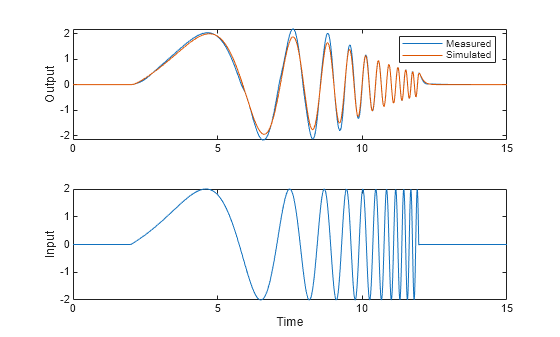
The general shape of the model response is similar to the measured output data, but there are some discrepancies. To get a better fit, you need to estimate the data in the spring stiffness lookup table.

Estimate Parameters Without Constraints

Perform parameter estimation without imposing any constraints on the spring stiffness values by using the sdoNonlinearSpringWithController_runEstimation helper function, which is provided at the end of the example. In this example, you use a small value for the maximum number of iterations for quick estimation, but you can edit the estimation function to change the maximum number of iterations if needed.

pOpt = sdoNonlinearSpringWithController_runEstimation("NoConstraint");

 Optimization started 2026-Jan-31, 01:56:32

                               max                     First-order 
 Iter F-count        f(x)   constraint    Step-size    optimality
    0     33      4.37709            0
    1     68     0.491881            0         1.16         3.15
    2    107     0.449389            0        0.148         2.81
    3    145     0.336414            0        0.233         2.28
    4    183     0.294876            0        0.167          3.6
    5    221     0.217276            0        0.286         1.23
    6    256     0.213377            0        0.305         1.03
    7    291     0.147624            0        0.297        0.868
    8    326     0.117138            0        0.259        0.789
Solver stopped prematurely.

fmincon stopped because it exceeded the iteration limit,
options.MaxIterations = 8.000000e+00.

Plot the estimated stiffness values against the corresponding deformation values. To get the deformation values, in the Simulink model, on the Modeling tab, in the Design section, click Model Workspace. The variable kBreakpoints stores the deformation values.

figure;
deformation = [ (-2 : 0.25 : -0.25)  (0.25 : 0.25 : 2)];
plot(deformation, abs(pOpt.Value), '-o');
xline(0);
xlabel('Deformation (m)')
ylabel('Stiffness (N/m)');

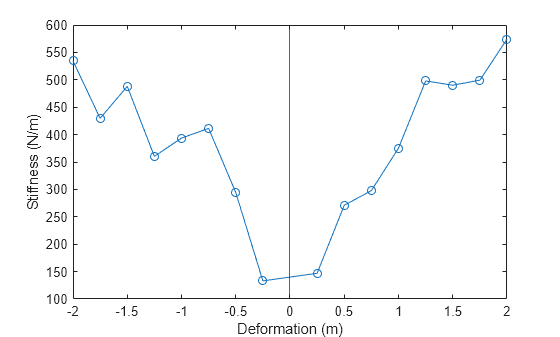
Based on physics, the spring stiffness values must monotonically decrease to the left of the line at Deformation = 0 and monotonically increase to the right of that line. Since the estimated spring stiffness values are not monotonic, you need to estimate the values again while imposing a monotonic constraint.

Estimate Parameters With Monotonic Constraint

Perform parameter estimation while imposing a monotonic constraint on the spring stiffness values by using the sdoNonlinearSpringWithController_runEstimation function.

pOpt = sdoNonlinearSpringWithController_runEstimation("WithConstraint");

 Optimization started 2026-Jan-31, 01:59:35

                               max                     First-order 
 Iter F-count        f(x)   constraint    Step-size    optimality
    0     33      4.37709            0
    1     70      1.91258            0        0.471          2.4
    2    109      1.17759      0.05572        0.213            2
    3    149     0.806554            0        0.119         1.79
    4    192     0.696669            0        0.038         1.72
    5    235     0.599947            0       0.0357         1.72
    6    275     0.348325            0        0.108         1.54
    7    312     0.075056            0         0.24         2.63
    8    351    0.0639096            0       0.0511         1.89
Solver stopped prematurely.

fmincon stopped because it exceeded the iteration limit,
options.MaxIterations = 8.000000e+00.

Plot the stiffness values against the corresponding deformation values.

figure;
deformation = [ (-2 : 0.25 : -0.25)  (0.25 : 0.25 : 2)];
plot(deformation, abs(pOpt.Value), '-o');
xline(0);
xlabel('Deformation (m)')
ylabel('Stiffness (N/m)');

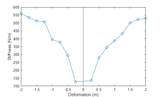
You can see that the estimated stiffness magnitudes now obey the monotonic constraint.

Update the model to use the estimated spring stiffness values using the sdo.setValueInModel function.

sdo.setValueInModel("sdoNonlinearSpringWithController","kTableData",pOpt.Value);

Stimulate the model using the chirp signal and compute the model response again using the computeModelResponse function.

[modelOutputTime,modelOutputData] = computeModelResponse(ChirpTime,ChirpInput,ChirpOutput);

Plot the input and output data. Plot the model response and compare it with the output data.

figure;
subplot(2,1,1);
plot(ChirpTime,ChirpOutput);
hold on;
plot(modelOutputTime,modelOutputData);
legend('Measured','Simulated');
ylabel('Output');

subplot(2,1,2);
plot(ChirpTime,ChirpInput);
ylabel('Input');
xlabel('Time');

The fit is significantly better compared to when you used the original spring stiffness values.

Validate Estimated Parameters

To validate the estimated spring stiffness values, first load the validation data set. This data set consists of pulse signals as inputs and outputs.

load("sdoNonlinearSpringWithController_Data.mat","PulseTime","PulseInput","PulseOutput");

Stimulate the model with the pulse signal and compute the model response by using the computeModelResponse function.

[modelOutputTime,modelOutputData] = computeModelResponse(PulseTime,PulseInput,PulseOutput);

Plot the input and output data. Plot the model response and compare it with the output data.

figure;
subplot(2,1,1);
plot(PulseTime,PulseOutput);
hold on;
plot(modelOutputTime,modelOutputData);
legend('Measured','Simulated');
ylabel('Output');

subplot(2,1,2);
plot(PulseTime,PulseInput);
ylabel('Input');
xlabel('Time');

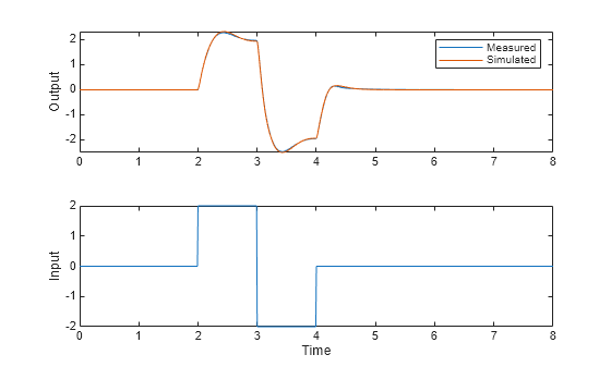
The plot shows that the model is able to generalize well to the validation data set.

Close the model.

close_system("sdoNonlinearSpringWithController",0);

Helper Functions

type computeModelResponse

function [modelOutputTime,modelOutputData] = computeModelResponse(time,input,output)
%Compute the model response.

%Create an experiment with the input and
%output data.
Exp = sdo.Experiment('sdoNonlinearSpringWithController');
% Specify the experiment input data used to stimulate the model.
Exp_Sig_Input = Simulink.SimulationData.Signal;
Exp_Sig_Input.Values    = timeseries(input,time);
Exp_Sig_Input.BlockPath = 'sdoNonlinearSpringWithController/In1';
Exp_Sig_Input.PortType  = 'outport';
Exp_Sig_Input.PortIndex = 1;
Exp_Sig_Input.Name      = 'Position Command';
Exp.InputData = Exp_Sig_Input;
% Specify the measured experiment output data.
Exp_Sig_Output = Simulink.SimulationData.Signal;
Exp_Sig_Output.Values    = timeseries(output,time);
Exp_Sig_Output.BlockPath = 'sdoNonlinearSpringWithController/Sensor Dynamics';
Exp_Sig_Output.PortType  = 'outport';
Exp_Sig_Output.PortIndex = 1;
Exp_Sig_Output.Name      = 'Position';
Exp.OutputData = Exp_Sig_Output;

% Create a model simulator from the experiment.
Simulator = createSimulator(Exp);

%Configure setup and restoration of the simulator.
Simulator = setup(Simulator, 'FastRestart', 'off');
% Add cleanup tasks to restore any changes after completion or termination.
% Use an anonymous function with no arguments that calls the restore method.
SimulatorCleanup = onCleanup(@() restore(Simulator));

%Run the model and store the model output.
Simulator = sim(Simulator);
simOutput = Simulator.LoggedData.logsout_MassSpringDamperWithController;
sigOutput = find(simOutput,'Position');
modelOutputTime = sigOutput.Values.Time;
modelOutputData = sigOutput.Values.Data;
end

type sdoNonlinearSpringWithController_runEstimation.m

function [pOpt,Info] = sdoNonlinearSpringWithController_runEstimation(type)
%SDONONLINEARSPRINGWITHCONTROLLER_RUNESTIMATION
%
% Perform parameter estimation for the sdoNonlinearSpringWithController model.
%
% This function returns the estimated parameter values, pOpt, and the estimation
% termination information, Info.
%
% The input argument, type, is either "NoConstraint" or
% "WithConstraint" and it determines whether a constraint is used in the estimation.
%

%Validate the input argument.
arguments
    type (1,1) string {mustBeMember(type, ["NoConstraint" "WithConstraint"])}
end

%% Open Model
open_system('sdoNonlinearSpringWithController')

%% Specify Model Parameters to Estimate
p = sdo.getParameterFromModel('sdoNonlinearSpringWithController', 'kTableData');
%Set the minimum and maximum values.
nonlinSpring = sprintf('%s\n%s', ...
    'sdoNonlinearSpringWithController/Nonlinear', ...
    'Translational Spring');
breakpoints = get_param(nonlinSpring,'deformation_vector');
breakpoints = sdo.getValueFromModel('sdoNonlinearSpringWithController',breakpoints);
p(1).Minimum(breakpoints > 0) = 0;
p(1).Maximum(breakpoints < 0) = 0;

%% Define Estimation Experiments
%
load('sdoNonlinearSpringWithController_Data.mat','ChirpTime','ChirpInput','ChirpOutput');
Exp = sdo.Experiment('sdoNonlinearSpringWithController');
% Specify the experiment input data used to stimulate the model.
Exp_Sig_Input = Simulink.SimulationData.Signal;
Exp_Sig_Input.Values    = timeseries(ChirpInput,ChirpTime);
Exp_Sig_Input.BlockPath = 'sdoNonlinearSpringWithController/In1';
Exp_Sig_Input.PortType  = 'outport';
Exp_Sig_Input.PortIndex = 1;
Exp_Sig_Input.Name      = 'Position Command';
Exp.InputData = Exp_Sig_Input;
% Specify the measured experiment output data.
Exp_Sig_Output = Simulink.SimulationData.Signal;
Exp_Sig_Output.Values    = timeseries(ChirpOutput,ChirpTime);
Exp_Sig_Output.BlockPath = 'sdoNonlinearSpringWithController/Sensor Dynamics';
Exp_Sig_Output.PortType  = 'outport';
Exp_Sig_Output.PortIndex = 1;
Exp_Sig_Output.Name      = 'Position';
Exp.OutputData = Exp_Sig_Output;


%%
% Create a model simulator from the experiment.
Simulator = createSimulator(Exp);

%% Configure Setup and Restoration of Simulator
%
% Set up the simulator.
Simulator = setup(Simulator, 'FastRestart', 'on');

% Add cleanup tasks to restore any changes after completion or termination.
% Use an anonymous function with no arguments that calls the restore method.
SimulatorCleanup = onCleanup(@() restore(Simulator));

%% Optimization Options
%
% Specify the optimization options.
Options = sdo.OptimizeOptions;
Options.Method = 'fmincon';
Options.MethodOptions.MaxIterations = 8;   % for short runs
Options.OptimizedModel = Simulator;

%% Create Estimation Objective Function
%
% To compute the estimation cost, create a function that you call at each
% optimization iteration.
%
% Use an anonymous function with one argument that calls either the 
% sdoNonlinearSpringWithController_optFcn_NoConstraint or the sdoNonlinearSpringWithController_optFcn_WithConstraint function.

switch type
    case 'NoConstraint'
        optimfcn = @(P) sdoNonlinearSpringWithController_optFcn_NoConstraint(P,Simulator,Exp);

    case 'WithConstraint'
        % Specify the design requirements to satisfy during optimization.
        Requirements = struct;
        Requirements.MonotonicVariable = sdo.requirements.MonotonicVariable;
        optimfcn = @(P) sdoNonlinearSpringWithController_optFcn_WithConstraint(P,Simulator,Exp,Requirements);
end

%% Estimate Parameters
%
% Call sdo.optimize with the estimation objective function handle,
% parameters to estimate, and optimization options as inputs.
[pOpt,Info] = sdo.optimize(optimfcn,p,Options);
end